Week 2 — Sep 21: Analytical Methods Development, the Modality Landscape, and Risk
Three things that have to be understood together before anything else in the course makes sense: how an analytical method actually gets developed and regulated, what is actually being made (the modality landscape), and how much evidence is enough (quality risk management).
(Lecture 2.) Week 1 argued that a method is a hypothesis about a molecule and that the discipline is built to revise it when the evidence says so. This week asks three questions that sit underneath everything else in the course: how does an analytical method actually get developed and regulated, what is actually being made, and how much evidence is enough? The third question is risk — assessed explicitly, not by reflex — and it’s the one this week is named for; the first two are the ground it stands on.
The one idea
A control strategy cannot be designed in the abstract — it is designed against a specific molecule, made by a specific process, measured by a method developed and validated for that purpose, with its own population of things that can go wrong. Before the course can teach how you measure something and how you control it, it has to teach what you are holding and how the method that measures it came to exist — then it can teach how much evidence is enough.
Analytical methods development and regulation
Every technique week for the rest of the term assumes a method already exists. This section is the one-page version of how it got there, so that assumption is never invisible:
Stage
What happens
Ties to
Analytical target profile (ATP)
State the requirement — analyte, matrix, range, accuracy/precision — before any column, wavelength, or probe is chosen
The regulatory expectation — captured in ICH Q14 — is that a method is designed against its validation targets and its analytical target profile from the start, not developed first and validated as an afterthought. Every worked method later in the course (chromatography, mass spec, spectroscopy) follows this same lifecycle; this is the only week that names it explicitly end to end.
What’s actually being made, and how much evidence is enough
Two more questions sit underneath every technique week: what is actually being made, and how much evidence is enough? Both get their own full treatment this week, in their own sections:
The modality landscape — a small molecule, a large molecule / biologic, and an advanced therapy compared side by side (size, manufacture, what “the molecule” even is, what purity means), plus why small molecule dominates entry-level hiring.
Quality risk management — the ICH Q9(R1) framework, the risk-management toolbox (FMEA, FTA, HACCP, HAZOP, risk ranking and filtering, Ishikawa/PHA, each with its own full walkthrough), and how a risk assessment becomes a control strategy.
The risk-homework thread
Three of the technique weeks later in the term — atomic spectroscopy, molecular spectroscopy, mass spectrometry — carry a risk-assessment assignment: take the method taught that week and build a method FMEA against a stated analytical target profile. The point is repetition: by the third checkpoint, scoring detectability should be a habit.
Where the analyst sits
Nobody hands you the modality landscape or the method-development lifecycle on day one — you infer them from the job posting, the SOPs on the shelf, and the first specification you’re asked to read. And in almost every method FMEA, the analyst is the only person in the room who knows the true detection score. A project manager can estimate severity; a process chemist can estimate occurrence; but whether the current controls would actually catch a failed extraction, a mis-integrated peak, a drifting calibration, or a co-eluting impurity before it reached a release decision is analytical knowledge, and if the analyst rounds it toward “we’d probably catch it,” the whole assessment is quietly wrong.
This is the STEAM “A” again: judgment about what the evidence can and cannot rule out. The refrain for the term — science → evidence → reduced uncertainty → control → regulatory confidence → patient trust — runs through method development above, and through the modality landscape and risk management in the sections that follow.
On the job
Read a job posting for an “Analytical Chemist I” or “QC Analyst” role and identify which column of the modality table it’s written against — the instrument list in the posting almost always gives it away.
Small molecule dominates entry-level hiring for a structural reason: there are simply more marketed small-molecule products, more generic and CDMO manufacturing sites, and more routine QC testing volume than for biologics or advanced therapies, which remain comparatively low-volume, specialised, and concentrated at fewer sites.
You will fill out, or be asked to sign off on, an FMEA far more often than you will build one from scratch — learn to read one critically before you learn to write one.
“Detection” is the column you’ll be asked about most, because you’re usually the only person in the room who actually knows what the running method would or wouldn’t catch. Don’t round it up to be agreeable.
A risk assessment that predates you (written by someone who’s since left) is still binding until it’s formally revisited — know how to find it, read it, and flag when it no longer matches reality.
For discussion
A job posting lists “HPLC, dissolution, ICP-MS” as required instruments. Which column of the landscape table is this role almost certainly in?
Why does “purity” require a panel of methods for a biologic but one method for a small molecule? Push past “it’s bigger” to the actual mechanism.
An advanced-therapy company is hiring far fewer analysts than a generic small-molecule manufacturer down the road, for a product that’s scientifically more sophisticated. Reconcile that with “the industry needs analytical skill.”
A method FMEA gives a mis-integration failure mode an RPN of 90 (S=9, O=2, D=5) and a wrong-diluent failure mode an RPN of 90 (S=5, O=3, D=6). Should they get the same attention? What does RPN hide here?
Your detection score for “co-eluting unknown degradant” depends on data you don’t have yet (forced degradation isn’t finished). How do you score it now, and what do you commit to?
The nitrosamine risk assessments concluded “no risk” for many products on the strength of a purge argument, with no confirmatory testing. When is a scientific argument enough, and when do you need the number?
Source note. Method-development framing follows ICH Q14 and ICH Q2(R2). See the modality landscape and risk management for their own sourcing. (Instructor: this session now absorbs what were two separate lecture weeks — confirm the pacing works in a single 3-hour slot.)
1 - What's Actually Being Made — the Modality Landscape
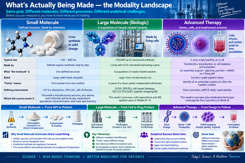
Before any technique week makes sense, the course needs to answer what is actually being made: a small molecule, a large molecule / biologic, and an advanced therapy compared side by side — size, manufacture, what “the molecule” even is, what purity means, and why small molecule dominates entry-level hiring.
The one idea
Before the course can teach how you measure something, it has to teach what you are holding — a small molecule, a large molecule, and an advanced therapy fail differently, are made differently, and demand entirely different definitions of “pure.”
What’s actually being made — the modality landscape
Before any of the technique weeks make sense, the course needs to answer a question that has to come first: what is actually being made?
The bottom rows are a thread the whole course pulls on: as a modality gets more complex, the “purity” question needs more methods to answer it, and each of those methods has to work harder to defend its own answer.
How each modality is made and tested
Small molecule — API synthesis and scale-up, then solid-dosage manufacturing (direct compression vs. granulation, compression, coating, packaging). Dissolution — the one routine test about the patient’s experience rather than the molecule’s identity — is covered later, in Week 9, alongside the other characterization techniques. The technique weeks that measure all of this — atomic spectroscopy, molecular spectroscopy, separations, specialized characterization, mass spectrometry — follow later in the term.
If you walk into a QC or analytical-development lab in this industry, the odds are strongly in favour of small molecule: tablets, capsules, and injectables built from defined organic synthesis still dominate the number of open analytical roles, which is why this course gives that column the most technique-week time and the other two their own depth here, up front, instead of spread across dedicated weeks. That is not a judgment about which modality matters more scientifically — it is a plain reflection of where the jobs are, and a course meant to get you ready for one should weight itself the same way.
Source note. The modality landscape follows standard pharmaceutical-technology and biopharmaceutical references; the jobs-market framing follows industry hiring-volume reporting (BioSpace, ACS C&EN annual employment surveys) rather than a single citable guideline. (Instructor: confirm current hiring-volume figures if citing numbers in lecture.)
1.1 - How an API Is Made — Synthesis and Scale-Up
The active pharmaceutical ingredient as a multi-step organic synthesis: route selection, why bench chemistry and plant chemistry are different disciplines, what changes — and what breaks — going from milligrams to tonnes, where ICH Q7 GMP begins in the route, and how the API’s final physical form sets up everything the next section does to it.
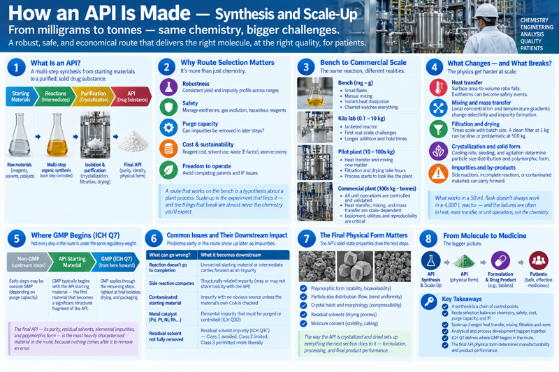
Before there is a tablet, there is a molecule, and before there is a molecule at commercial scale, someone has to have proven — repeatedly, at increasing scale — that the same reaction that worked in a 50 mL flask still works in a 4,000 L reactor. That proof is process research and scale-up, and it is where most of an API’s eventual impurity profile and physical form get decided.
The one idea
A route that works on the bench is a hypothesis about a plant process. Scale-up is the experiment that tests it — and the things that break are almost never the chemistry you’d expect.
A synthesis is a chain of control points
An API is built from starting materials through a defined sequence of reactions, each producing an isolable intermediate, until the final step delivers the API itself — usually followed by a purification (crystallization, sometimes chromatography) that fixes its final form. Every step is a place where things can go right or wrong:
What can go wrong at a step
What it becomes downstream
Reaction doesn’t go to completion
Unreacted starting material or intermediate carries forward as an impurity
A side reaction competes
A structurally related impurity, sometimes sharing the API’s toxicity, sometimes not
A contaminated or off-spec starting material
An impurity with no obvious source unless the material’s own CoA is checked
A metal catalyst (Pd, Pt, Ni, Rh…)
An elemental impurity that has to be purged or controlled — the direct link to ICH Q3D testing, the week atomic spectroscopy is taught
Residual reaction solvent not fully removed
A residual solvent impurity (ICH Q3C), classed by toxicity (Class 1 avoided, Class 2 limited, Class 3 permitted more liberally)
None of this is visible in the finished white powder. It is found — or missed — by the analytical methods built around the route, which is why route chemistry and analytical method development happen together, not in sequence.
Choosing a route is not just chemistry
Process research doesn’t take the first route that works; it evaluates candidate routes against criteria that have nothing to do with whether the reaction is elegant:
Robustness — does the yield and impurity profile hold up across the ranges of temperature, concentration, and reagent quality a plant will actually see, or does it need bench-level precision?
Safety — exotherms, gas evolution, unstable intermediates, reagents that are fine in a fume hood and dangerous in a jacketed reactor holding hundreds of litres.
Purge capacity — can later steps (crystallizations especially) reliably wash an impurity out, so an early imperfection doesn’t have to be perfect?
Cost, atom economy, and green chemistry — solvent volumes, reagent cost, waste generated per kilogram of API, and increasingly a formal E-factor target.
Freedom to operate — does the route avoid a competitor’s process patent?
A route redesigned late in development to fix one of these is common, and every redesign reopens the impurity and degradation picture — which is exactly the “moving target” that makes a systematic, comparable analytical program non-negotiable across route changes.
Bench → kilo lab → pilot plant → commercial plant
The same reaction run at four scales is not the same experiment, because the physics around the chemistry changes with vessel size in ways the flask never revealed:
Scale
Typical batch
What’s now different
Bench
mg – g
Fast manual mixing, instant heat dissipation, chemist watches every addition
Kilo lab
0.1 – 10 kg
First real jacketed reactor, first agitator design, first taste of longer addition and hold times
Pilot plant
10 – 100s kg
Heat transfer and mixing efficiency now scale-dependent, not assumed; filtration and drying take hours, not minutes
Commercial plant
100s kg – tonnes
Every unit operation (charge, react, quench, extract, crystallize, filter, dry) is now a controlled, validated process step
Why scale-up breaks things that bench chemistry never revealed:
Surface-area-to-volume ratio falls as vessels get bigger, so heat that dissipated instantly in a flask now has to be removed through a jacket — an exotherm that was a non-event on the bench can become a runaway or a safety incident in a reactor.
Mixing and mass transfer get harder, not easier — a reagent added over seconds by hand goes in over hours through a dip pipe, so local concentration and temperature gradients appear that a flask never had, changing selectivity and impurity formation.
Filtration and drying times scale with cake depth and batch size, not linearly with batch mass — a crystallization that filters cleanly at 1 kg can be impractically slow, or dry unevenly, at 500 kg.
Crystallization control becomes the whole ballgame for the API’s final physical form — cooling rate, seeding, and agitation at scale determine particle size distribution and polymorphic form, both of which the next section inherits directly: they decide whether the API even flows and compresses well enough for direct compression, or whether it needs granulating first.
Where GMP begins in the route
Not every step in the synthesis is manufactured under the same regulatory weight. ICH Q7 draws a line at the API starting material — the raw material or intermediate that becomes a significant structural fragment of the API — and GMP applies from that point forward, tightening as the route approaches the final isolation. The logic is purge capacity again: an error early in the route can still be removed by a later purification step; an error in the final crystallization, drying, or micronization reaches the patient with nothing left to catch it. This is also why the final isolated API — its purity, its residual solvents, its elemental impurities, its polymorphic form — is the single most heavily analytically characterised material in the whole route.
Where the analyst sits
The chemist who ran the route on the bench is rarely the person defending it in a regulatory filing five years later at commercial scale. The record that survives — validation batches, in-process specifications, impurity qualification data — has to speak for a process that changed as it scaled. Reading that record and asking does this impurity limit still make sense given how the route actually runs today is analytical judgment, not chemistry.
For discussion
A palladium-catalysed coupling step is three steps before the final API isolation. Why might the elemental-impurity risk still be considered high, even with two purifications in between?
A crystallization that gave a single, reproducible polymorph at kilo-lab scale gives a mixture of two polymorphs at pilot-plant scale, with no change to the recipe on paper. What changed, and how would you find out?
Process research chooses a lower-yielding route because it avoids a Class 1 residual solvent entirely. Was that the right trade, and what would change your answer?
Source note. Route selection and scale-up follow standard process-chemistry texts (Anderson, Practical Process Research & Development) and the Q3C residual-solvent classes. GMP scope follows ICH Q7. (Instructor: add a specific worked route once course examples are finalised.)
1.2 - From Powder to Tablet — Solid-Dosage Manufacturing
Turning the API powder into a tablet the patient can swallow: direct compression versus dry (roller-compaction) and wet (fluid-bed) granulation, compression and coating, and the packaging that protects what all of it achieved — bottles, foil blisters, and capsules — with each process choice justified against the API’s own properties and the stability / quality-by-design case behind it.
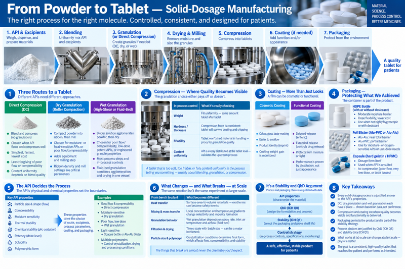
The previous section ended with the API’s final physical form — particle size, flow, compressibility, moisture sensitivity — decided by how it was crystallised and isolated. Everything in this section is downstream of that: the API’s own properties decide which manufacturing route is even available, before a single formulation decision is made.
The one idea
Every solid-dosage process is a justified answer to one question: given what this API actually is — how it flows, how it compresses, what degrades it — what is the least-handling route to a tablet that still meets its specification, batch after batch?
Three routes to a tablet, in order of how much they touch the powder
Route
What happens
When it’s chosen
What it costs you
Direct compression (DC)
API and excipients blended, then compressed straight into tablets — no intermediate agglomeration step
The API already flows and compresses well at the required dose; the simplest, cheapest, fastest route
Least forgiving of a poorly flowing or poorly compressible API; content uniformity is entirely dependent on blend quality
Dry granulation (roller compaction)
Powder is compacted into a ribbon between rollers, then milled into granules
API is moisture- or heat-sensitive, or doesn’t flow/compress well enough for DC, but can’t tolerate wet processing
Adds equipment and a milling step; ribbon density and mill settings become new critical parameters
Wet granulation (high-shear or fluid-bed)
A binder solution or suspension agglomerates the powder into granules, which are then dried
Poor flow or compressibility, low-dose potent APIs that need better content uniformity, or where granule properties must be engineered
Adds a drying step (moisture must come back out); the most process steps, the most in-process controls, the most that can go wrong
Fluid-bed granulation is the wet route worth naming specifically: the powder bed is fluidised in a stream of air while binder solution is sprayed in, and the granules are dried in the same vessel without transferring the batch — one piece of equipment doing agglomeration and drying together, which reduces handling but makes airflow, spray rate, and inlet-air temperature the parameters that decide whether the granule comes out right.
Compression and the properties it exposes
Whichever route produced the material — powder blend or granules — it is compressed into tablets, and compression is where the granulation choice either pays off or doesn’t:
In-process control
What it’s really checking
Weight
Fill uniformity — is the die filling the same amount, tablet after tablet?
Hardness / thickness
Compression force is consistent, and the tablet will survive coating and shipping
Friability
The tablet won’t shed material in handling — a proxy for how well the granulation held together
Content uniformity
The API is evenly distributed at the tablet level, not just the blend level — the test that ultimately validates the whole upstream route
A tablet that is too soft or too friable is usually a granulation problem revealing itself late; a tablet with poor content uniformity is usually a blending or flow problem revealing itself even later still. Compression is the first point any of this becomes visible as a number.
Coating — cosmetic, or a control
A film applied to the compressed tablet does one of two different jobs:
Cosmetic / taste-masking — colour, gloss, ease of swallowing, identity (colour and imprint) for the patient and pharmacist. Coating weight gain is tracked, but performance isn’t riding on it.
Functional coating — delayed-release (enteric, survives the stomach) or extended-release (controls the rate the drug is available at all). Here the coating is the mechanism, and dissolution becomes the test that decides whether the product works, not just whether it looks right.
Packaging — protecting what the process just achieved
Everything upstream — the API’s stability, the tablet’s moisture sensitivity, whether the coating is intact — is only as good as the container that ships it:
The API is not highly hygroscopic or photosensitive, or a desiccant closes the gap
Foil blister (Alu-PVC or Alu-Alu)
Alu-Alu is close to a total moisture/oxygen barrier; Alu-PVC is a partial one
Alu-Alu for genuinely moisture- or oxygen-sensitive APIs; Alu-PVC where the risk is lower and unit-dose presentation still matters
Capsule (hard gelatin / HPMC)
The dosage form itself, packaged in bottle or blister
The API is unsuited to compression at all — poor compressibility, very low dose needing a carrier, or a taste that tableting can’t mask
The justification is a stability and QbD argument, not a preference
None of the choices above are made on convenience. Each is defended with data and traced back to a control strategy:
The route (DC vs. dry vs. wet granulation) is justified by the API’s measured flow, compressibility, and moisture/heat sensitivity — a quality-by-design argument under Q8: the process is designed around the material’s known properties so that a conforming batch is the expected outcome, not a hoped-for one.
The packaging is justified directly by stability data under ICH Q1 — a hygroscopic API that shows significant change in an open-dish humidity study earns an Alu-Alu blister or a desiccant bottle; a photosensitive one earns an opaque bottle or overwrap, backed by Q1B photostability data.
Container-closure integrity is itself a tested attribute, not an assumption — it is part of what the stability program is confirming batch after batch, on the shelf, for the life of the product.
Put together, the manufacturing route and the pack are two halves of one answer to the same question this week’s risk-management framework asks of everything it touches: what could go wrong with this specific molecule, and what does the process or the pack have to do about it?
Where the analyst sits
None of the choices above are visible in a finished tablet by inspection. A tablet made by direct compression and one made by wet granulation can look identical and perform very differently under stress — which is exactly why the in-process controls in the tables above exist, and why a batch record reader needs to know which control is protecting against which upstream decision.
For discussion
A roller-compacted formulation and a wet-granulated formulation both meet release specifications for the same product. What stability or robustness question would you still want answered before picking one for commercial launch?
An API is reformulated from a bottle with desiccant to an Alu-Alu blister after a stability failure. What does that change tell you about the API, and what data would have predicted it before the failure?
A functional (extended-release) coating passes every appearance and weight-gain check, but the batch still fails dissolution. Where would you look first?
Source note. Solid-dosage unit operations follow standard pharmaceutical-technology texts (Aulton, Pharmaceutics: The Design and Manufacture of Medicines). QbD justification follows ICH Q8; packaging justification follows ICH Q1.
1.3 - How the Toolkit Scales Up — Large Molecules & Biologics
How the analytical toolkit scales up to biologics: recombinant manufacture and the control points along it, the monoclonal-antibody CQA panel, potency as a biological measurement, binding kinetics by SPR/BLI, particles and aggregation, and comparability (ICH Q5E) — the large-molecule column of the modality landscape, in depth.
This section fills in the large molecule column of the modality landscape table above. A small molecule’s “purity” is one number from one method; a protein’s is a dozen partly-independent attributes, and its potency is a biological measurement, not a chemical one. The separations and mass-spectrometry methods that read most of this panel are taught in full — with a worked case that starts here — in Separation Methods and Mass Spectrometry.
The one idea
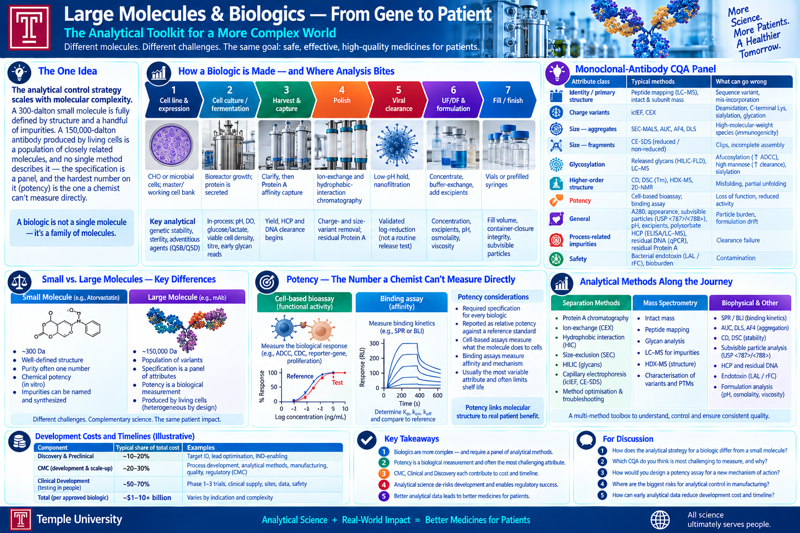
The analytical control strategy scales with molecular complexity. A 300-dalton small molecule is fully defined by structure and a handful of impurities. A 150,000-dalton antibody produced by living cells is a population of closely related molecules, and no single method describes it — the specification is a panel, and the hardest number on it (potency) is the one a chemist can’t measure directly.
How a biologic is made — and where analysis bites
Step
What happens
Analytical control
Cell line & expression
A gene inserted into CHO (or microbial) cells; a master/working cell bank
Fill volume, container-closure integrity, subvisible particles
Contrast with small-molecule manufacturing: defined reactions, isolable intermediates, impurities you can name and synthesise. Here the “impurities” are the cells’ own proteins and DNA, and the product itself is heterogeneous by design.
The monoclonal-antibody CQA panel
Attribute class
Methods
What can go wrong
Identity / primary structure
Peptide mapping (LC–MS), intact & subunit mass — taught in full
Potency is a required specification for every biologic, and usually the one that limits shelf life. It is a biological measurement of function, reported as relative potency against a reference standard:
Cell-based bioassays — proliferation, reporter-gene, ADCC/CDC — measure what the molecule does to cells, often read out by flow cytometry (counting labelled cells or measuring a fluorescent reporter one cell at a time — Week 9 teaches the technique in full; the advanced-therapies section introduces its CAR-T application). Biologically relevant, and variable: geometric %CV of 10–20% is normal.
Binding assays — ELISA, and kinetic methods (SPR / Biacore, BLI / Octet) measuring association and dissociation rate constants and affinity (KD) — are more precise but measure binding, not function; acceptable when binding is shown to predict activity.
The reference standard is itself a stability-limited material with a potency value; when it is replaced, a bridging study re-anchors the scale, and any drift there propagates into every future result.
Particles and the immunogenicity link
Protein aggregates and subvisible particles are associated with immunogenicity. Control spans three size regimes with different methods, and no single method covers the range: submicron (DLS), subvisible ~1–100 µm (light obscuration, flow imaging microscopy), and soluble oligomers (SEC, AUC, AF4). Orthogonality is the theme: you believe an aggregation result when methods with different failure modes agree.
Comparability — the analytical argument
Every manufacturing change — a new site, a bigger bioreactor, a formulation tweak — raises the question: is it still the same product?ICH Q5E answers it with a tiered, risk-based analytical comparison: the more an attribute matters to safety and efficacy, the more sensitive the method and the tighter the acceptance criterion. Biosimilars run the same logic in reverse: analytical similarity to the reference product is the foundation of the whole abbreviated pathway.
Worked case — a charge-variant shift after a process change
A mAb process moves to a larger bioreactor. Post-change lots show acidic charge variants up from 18% to 26% by icIEF. Everything else in the panel is comparable, and potency is unchanged. Peptide mapping localises the extra acidic species to increased deamidation at a known site; HDX-MS and an FcRn binding assay confirm it doesn’t affect binding or recycling. The resolution: comparable on function, a localised and characterised chemical difference within prior experience, accepted with a tightened in-process control. Had potency moved, or had the variant been uncharacterised, it would have needed a PK bridging study.
Where the analyst sits
With a panel this large, the judgment is triage — which attribute is the one that would actually harm a patient if it drifted. And potency forces a specific call the rest of the course doesn’t: how much assay variability is acceptable when the attribute is function itself. That is the STEAM “A” at its most consequential.
On the job
A large-molecule CQA panel report will land on your desk as a dozen numbers from a dozen instruments — your first real skill is triage: which one, if it drifted, would you refuse to release on?
Expect your first exposure to potency assays to be as a reader of a bioassay report, not a runner of one — cell-based assays are typically run by a specialized team, but every analyst on the product needs to interpret the %CV and the reference-standard bridging history.
“Comparable” on a Q5E comparability exercise is a conclusion you’ll be asked to defend line by line, attribute by attribute — not a single yes/no you can wave at.
For discussion
A mAb’s potency assay has a geometric %CV of 18%. The specification is 80–125% relative potency. How many replicates do you need to make a confident release decision, and what does that cost per batch?
SEC says 2.0% aggregate; AUC says 3.5%. Which do you report, and how do you resolve the discrepancy?
In the worked case, what would have made you insist on a PK bridging study despite unchanged potency?
Biosimilar developers argue analytical methods are now sensitive enough to make some comparative clinical trials unnecessary. Where is that argument strong, and where does it break?
Source note. Manufacturing and control follow standard biopharmaceutical references and ICH Q5A–Q5E, Q6B, and Q11. Potency and bioassay design follow USP ⟨1032⟩–⟨1034⟩; particles follow USP ⟨787⟩/⟨788⟩/⟨1787⟩. Comparability follows ICH Q5E; biosimilar analytical similarity follows FDA/EMA biosimilar guidance. Endotoxin: USP ⟨85⟩/⟨86⟩. (Instructor: confirm current biosimilar analytical-similarity expectations.)
1.4 - The Analytical Frontier — Advanced Therapies
The analytical frontier, taught with its two defining instruments in full: flow cytometry (principles, panel design, gating, and its use for CAR-T identity/purity/potency) and ddPCR (vector genome titre, vector copy number) — plus gene therapy (AAV, full/empty capsid), mRNA-LNP, oligonucleotides, and NGS. Where batch size shrinks toward one and the analyst defines the method and the specification at the same time as the product.
This section fills in the advanced therapy column of the modality landscape table above. Large molecules were a population of one designed molecule. Advanced therapies push further: the “product” can be a virus, a strand of mRNA inside a lipid particle, or a single patient’s own cells — and the batch can be one.
The one idea
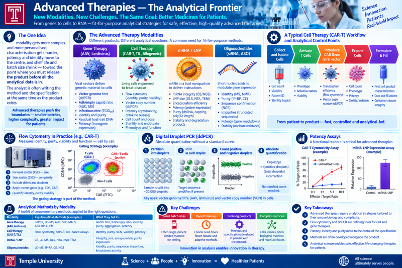
As a modality gets more complex and more personalised, characterisation gets harder, potency and identity move to the centre, and shelf life and batch size shrink — toward the point where you must release the product before all the analytical data is in. The analyst is often writing the method and the specification at the same time as the product exists.
Flow cytometry, in practice
Flow cytometry is the defining instrument of cell therapy, and it’s worth understanding mechanically, not just as a table entry — Week 9 gives it the full technique-lecture treatment (instrumentation, controls, and its reach beyond cell therapy); this is the CAR-T-specific application:
The principle. Cells in suspension flow single-file past a laser. Each cell scatters light (forward scatter ≈ size, side scatter ≈ granularity/complexity) and, if labelled with fluorescent antibodies or dyes, emits at specific wavelengths — measured cell by cell, thousands per second.
Panel design. Each fluorophore needs a distinct enough emission to be resolved from the others (spectral overlap is corrected by compensation or, in newer spectral cytometers, unmixing algorithms); a panel is built around the specific surface markers (CD antigens) that define the cell population of interest.
Gating. Data is filtered sequentially — first to exclude debris and doublets, then to select the population of interest by marker combination — and the order and logic of the gates is part of the method, not an analysis afterthought; two analysts gating the same raw data differently can report different results from identical instrument output.
What it measures for CAR-T:identity and purity (percentage of cells expressing the target CD markers), viability (live/dead stains), transduction efficiency (percentage expressing the introduced CAR construct), and — via a functional assay read out on the cytometer — a component of potency.
ddPCR, in practice
Digital droplet PCR partitions a sample into tens of thousands of nanoliter droplets, runs PCR in each independently, and counts how many droplets are positive versus negative for the target sequence — turning a continuous amplification signal into absolute molecule counts, with no reference standard curve required.
Vector genome titre — for AAV and lentivirus, the absolute count of vector genomes per mL, the number that anchors dose.
Vector copy number (VCN) — for transduced cells, how many copies of the therapeutic gene integrated per cell; too low and there’s insufficient expression, too high raises a genotoxicity concern (insertional mutagenesis).
Why ddPCR over qPCR here: absolute quantitation without a standard curve matters when reference materials are scarce or don’t yet exist — exactly the advanced-therapy situation.
The modalities and their control
Modality
Made by
Characteristic analytical panel
Gene therapy (AAV, lentivirus)
Transient transfection or packaging cell lines; downstream chromatography
Vector genome titre (ddPCR), capsid identity (LC–MS), full/empty capsid ratio (AUC, charge-detection MS, AEX-HPLC, cryo-TEM), infectious titre (TCID50), aggregation (SEC-MALS, AUC), residual host-cell DNA / plasmid / helper functions, replication-competent virus, potency (transgene expression and function)
Flow cytometry (above); vector copy number (ddPCR, above); potency (cytotoxicity, cytokine release); rapid sterility and endotoxin; cell count and dose
mRNA / LNP
In-vitro transcription → LNP formulation
mRNA integrity (CE / on-chip electrophoresis), 5′ cap and poly(A) tail analysis (LC–MS), dsRNA impurity, encapsulation efficiency and mRNA content (RiboGreen), lipid identity and quantitation (HPLC-CAD, LC–MS), particle size / PDI (DLS), zeta potential, in-vitro expression potency
Oligonucleotides (ASO, siRNA)
Solid-phase synthesis
The bridge between small and large: IEX- and RP-HPLC, LC–MS for identity and sequence-related impurities (n−1, n+1, depurination), CE
The recurring problems
Potency, again — but worse. For a living or self-assembling product, potency is central and hard: a cell-therapy cytotoxicity assay or an AAV transgene-function assay carries large variability, and there is often no validated reference material.
Identity of an assembly. When the “molecule” is a capsid carrying a genome, or a lipid particle carrying mRNA, identity is a set of orthogonal reads, not one spectrum — extending the native-MS discussion to whole viral particles.
Release before the data. A 14-day sterility test does not fit a 3-day autologous product — hence rapid microbial methods (rapid sterility, ATP bioluminescence, NAT-based mycoplasma) and, sometimes, conditional release with follow-up.
NGS as the new cross-cutting tool. Next-generation sequencing now does vector and plasmid identity/integrity, mRNA sequence confirmation, cell-line characterisation, and adventitious-agent detection — increasingly replacing in-vivo assays.
The frameworks are still forming. FDA (OTP) and EMA (ATMP / CAT) guidance, and the accelerated pathways these products often use, are evolving faster than the compendia — a lesson about working on a moving regulatory target that the chemometrics/AI week develops later in the term.
Where the analyst sits
With almost no reference materials, forming guidance, a batch size that can be one, and a clock that can be days, the analyst on an advanced therapy is doing the whole of Week 1 at once: choosing what to measure, developing the method, setting the specification, and defending all three. It is judgment under maximum uncertainty, and it is the STEAM “A” with the training wheels off.
On the job
Flow cytometry gating is one of the first places a new hire’s independent judgment shows up on a report — expect your gating scheme to be reviewed by someone more senior before your first result goes on a batch record.
If you can read a ddPCR report and explain why it doesn’t need a standard curve the way qPCR does, you’re ahead of most new hires walking into a cell-and-gene-therapy lab.
“Release before the data” is not a corner being cut — it’s a defined, validated pathway with its own paperwork (conditional release, follow-up commitments); know where to find that paperwork before you need it.
Reference materials you’d expect to just exist (a certified AAV capsid standard, a certified CAR-T potency standard) often don’t — part of the job is knowing how a lab qualifies its own in-house reference material when nothing external exists.
For discussion
An AAV lot has a full/empty capsid ratio just outside spec, but infectious titre and potency are both in range. Would you release it? What would you want to know first?
Two analysts gate the same flow-cytometry raw data differently and get different purity numbers. Whose is “right,” and how would a lab prevent this in practice?
A CAR-T cytotoxicity assay has a %CV of 30% and there is no certified reference material. How do you set a defensible specification anyway?
NGS can confirm mRNA sequence, detect adventitious agents, and characterise a cell line. What does it not tell you that a targeted assay still would?
Source note. Gene- and cell-therapy analytics follow USP ⟨1046⟩/⟨1047⟩, the emerging AAV and cell-therapy chapters, and FDA OTP and EMA ATMP guidance; flow cytometry follows standard cytometry references (Shapiro, Practical Flow Cytometry) and USP ⟨1027⟩; ddPCR follows the digital-PCR literature. mRNA-LNP follows the vaccine and mRNA-therapeutic analytical literature; oligonucleotides follow the OBP/USP oligonucleotide work. Rapid microbial methods follow USP ⟨1071⟩/⟨1223⟩ and Ph. Eur. 5.1.6 / 2.6.27. (Instructor: this field moves monthly — confirm the current guidance set; a live flow-cytometry gating demo, even on public example data, lands far better than the table alone.)
2 - Quality Risk Management — How Much Evidence Is Enough
ICH Q9(R1) as a loop, not a form: the risk-management toolbox (FMEA, FTA, HACCP, HAZOP, risk ranking and filtering, Ishikawa/PHA), FMEA in action, and how a risk assessment becomes a control strategy — worked through the nitrosamine risk assessments.
The one idea
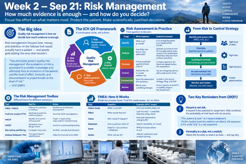
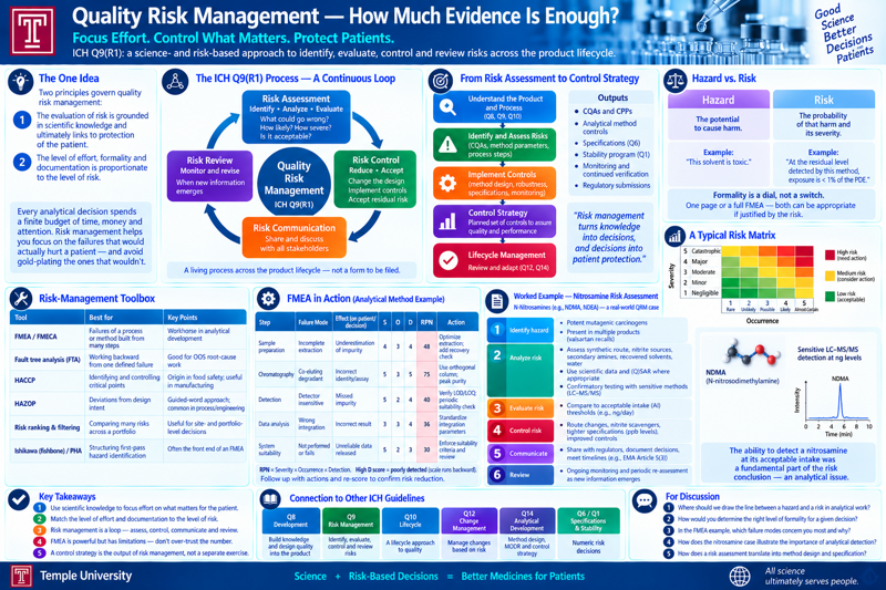
Two principles govern quality risk management: the evaluation of risk is grounded in scientific knowledge and ultimately links to protection of the patient; and the level of effort, formality, and documentation is proportionate to the level of risk.
Every analytical decision spends a finite budget of time, money, and attention. Risk management is how you point that budget at the failures that would actually hurt a patient, and stop gold-plating the ones that wouldn’t. It is the machinery behind “scientifically justified” — the phrase that appears in almost every ICH guideline and is doing a lot of quiet work.
The ICH Q9 framework
ICH Q9(R1) — Quality Risk Management (the R1 revision, adopted 2023, added guidance on subjectivity, the hazard-versus-risk distinction, formality, and risk-based decision-making). The process is a loop, not a form:
Stage
What happens
Analytical example
Risk assessment — identification
What could go wrong?
A co-eluting degradant is not resolved from the API
Risk assessment — analysis
How likely, how severe, how detectable?
Estimate occurrence from forced-degradation data; severity from the degradant’s qualification threshold; detection from method specificity
Risk assessment — evaluation
Is that acceptable against defined criteria?
Compare against a risk threshold agreed before the assessment
Risk control — reduction
Change the design to lower likelihood or raise detection
Switch to an orthogonal column; add a peak-purity check
Risk control — acceptance
Some residual risk is accepted, explicitly and on the record
Document the residual and the justification
Risk communication
The assessment and decisions are shared with everyone who acts on them
The control strategy, the filing, the SOP
Risk review
Revisit when something changes
A new impurity at month 9 of stability reopens the assessment
Two ideas from Q9(R1) matter for the analyst:
Hazard is not risk. A hazard is the potential to cause harm; risk combines the probability of that harm with its severity. “This solvent is toxic” is a hazard statement; “at the residual level this method can detect, the exposure is X% of the PDE” is a risk statement.
Formality is a dial, not a switch. A one-line rationale, a risk-ranking table, and a full cross-functional FMEA are all valid quality risk management — the guideline asks you to match the formality to what is at stake, and to say why.
The toolbox
Each tool below gets its own full walkthrough — mechanics, a worked analytical example, and where it breaks down:
Failure Mode and Effects Analysis decomposes a method or process into steps, and for each step asks: what could fail (failure mode), what would that do (effect), why would it happen (cause), and how would we catch it (controls). Each mode is scored:
Risk Priority Number = Severity × Occurrence × Detection
Severity — how bad the effect is for the patient or the decision (a wrong release decision scores high; a re-run scores low).
Occurrence — how often the cause is expected to produce the failure.
Detection — how likely the existing controls are to catch it before it matters. High detection score = poorly detected — this scale runs backward, and it is where most FMEAs go wrong.
Modes with a high RPN, or a high severity regardless of RPN, get an action; then the mode is re-scored to show the action worked. The number is easy to game and easy to over-trust — see the full FMEA walkthrough for a worked multi-failure-mode example and the known weaknesses worth teaching so students don’t over-trust it.
From risk assessment to control strategy
A control strategy is the planned set of controls — derived from current product and process understanding — that assures performance and quality. It is the output of risk management, not a separate exercise:
Attribute risk assessment decides which quality attributes are critical (CQAs) and therefore need a specification and a method.
Method risk assessment (an FMEA against the analytical target profile) decides which method parameters need to be controlled, and how tightly — this is where a robustness study is a risk-control activity, not a validation checkbox.
The specification (Q6) and the stability program (Q1) are risk decisions in numeric form.
Worked example — nitrosamine risk assessments. Between 2018 and 2023 every marketing authorization holder had to assess every product for the risk of N-nitrosamine impurities (NDMA, NDEA, and drug-specific nitrosamines), triggered by the valsartan recalls. The assessment is a textbook QRM: identify the hazard (potent mutagenic carcinogens), analyze the risk (synthetic route, nitrite sources, secondary amines, recovered solvents, water; then confirmatory testing), control it (route changes, nitrite scavengers, tightened limits at ppb levels), and communicate it (to the agency, on a deadline). It also shows the analyst’s exposure directly: the risk conclusion depended entirely on whether a method existed that could see a nitrosamine at its acceptable intake — a detection problem.
Source note. Risk management is anchored in ICH Q9(R1), with ICH Q8(R2), Q10, and Q14. FMEA methodology follows IEC 60812 and the AIAG-VDA FMEA handbook. The nitrosamine case follows the EMA/FDA guidance and Article 5(3) referral outcomes. (Instructor: confirm the Q9(R1) adoption date and current EMA nitrosamine guidance revision.)
2.1 - FMEA in Detail — Scoring, Scaling, and Where It Breaks
Failure Mode and Effects Analysis worked end to end on an HPLC assay method: the RPN formula, a full failure-mode table with a before/after action, why detection runs backward, and the known weaknesses that make RPN easy to over-trust.
The one idea
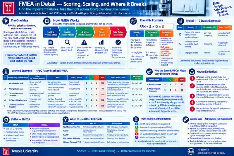
RPN is a prioritization tool, not a measurement. It tells you which failure mode to look at first — it does not tell you how much worse one failure mode is than another, and treating it like it does is the single most common way an FMEA goes wrong.
Mechanics
Failure Mode and Effects Analysis decomposes a method or process into steps, and for each step asks: what could fail (failure mode), what would that do (effect), why would it happen (cause), and how would we catch it (controls)? Each mode is scored on three independent 1–10 scales and multiplied:
Risk Priority Number = Severity × Occurrence × Detection
Severity — how bad the effect is for the patient or the decision. A wrong release decision (a failing batch shipped, or a good batch scrapped) scores high; a re-run that costs a day scores low.
Occurrence — how often the cause is expected to produce the failure, from historical data or, absent that, engineering judgment.
Detection — how likely the existing controls are to catch the failure before it matters. High detection score = poorly detected — this scale runs backward from the other two, and it is where most FMEAs go wrong: a “10” means “we would almost certainly miss this,” not “we’d definitely catch it.”
Modes with a high RPN, or a high severity regardless of RPN, get a corrective action; the mode is then re-scored to show the action actually moved the number, not just noted “action taken.”
Worked example — an HPLC assay method
Failure mode
Effect
Cause
Current control
S
O
D
RPN
Action
Re-scored RPN
Mis-integrated peak
Wrong reported assay value
Manual integration override without documented rationale
Similar-looking bottles stored adjacent on the bench
Analyst training
6
3
5
90
Segregate diluent storage; barcode-scan verification at weigh-in
6 × 3 × 2 = 36
Column-to-column carryover
Ghost peak misread as an impurity
Insufficient wash gradient between injections
None — relies on visual inspection
5
5
8
200
Add a blank injection after each sample series; extend wash time
5 × 5 × 3 = 75
Drifting calibration curve
Systematic bias in reported result
Standard degraded between preparation and use
System suitability at run start only
9
2
6
108
Add a mid-run suitability check; shorten standard hold time
9 × 2 × 3 = 54
Co-eluting unknown degradant
Impurity result reported low
Insufficient resolution between API and degradant
Resolution check in system suitability
9
3
4
108
Switch to an orthogonal column for confirmatory testing
9 × 3 × 2 = 54
Two things worth noticing in this table: the carryover mode (RPN 200) outranks the drifting-calibration mode (RPN 108) even though a wrong release decision from a drifting curve is arguably worse — because carryover’s detection score was so bad (8: nobody was actually looking for it). That is RPN doing its job: surfacing the blind spot, not just the scariest-sounding failure.
Why the same RPN can mean very different things
Failure mode
S
O
D
RPN
A
9
2
5
90
B
5
3
6
90
Both score 90. Mode A is a rare but severe failure that’s moderately well detected; mode B is a more frequent, less severe failure that’s poorly detected. A severity-first reviewer would act on A first regardless of the tied RPN — which is exactly the argument for not ranking a whole FMEA by RPN alone, and for flagging any mode with severity ≥ 9 for action independent of its RPN.
FMEA vs. FMECA
FMECA adds a formal criticality analysis on top of FMEA — instead of (or alongside) the RPN product, each failure mode’s criticality is assessed against a defined severity/probability matrix, often with failure-mode ratios when one cause can produce several distinct failure modes. In practice, most analytical-development FMEAs are really FMECAs in miniature: teams already flag “any severity ≥ 9 regardless of RPN” as an action trigger, which is a criticality rule, not a pure RPN rule.
Known weaknesses — worth teaching so students don’t over-trust the number
RPN is an ordinal product treated as if it were interval data; an RPN of 100 is not “twice as bad” as 50, and — as shown above — different (S, O, D) triples give the same RPN with very different meaning.
Detection and occurrence are often guessed. Q9(R1) explicitly flags this subjectivity and asks for it to be managed (defined scales, cross-functional scoring, documented assumptions).
Many programs now supplement or replace RPN with a severity-first criticality matrix, or with risk ranking and filtering when comparing failure modes across unrelated processes.
When to reach for something else
FMEA decomposes one process step by step and scores every mode on the same three scales — it’s the right tool when the process is defined and you’re building or revising its control strategy. Reach for fault tree analysis instead when you’re working backward from a failure that has already happened and need to trace its root cause; reach for risk ranking and filtering when you’re comparing risks that don’t share a process or a scale at all.
2.2 - Fault Tree Analysis — Working Backward From a Failure
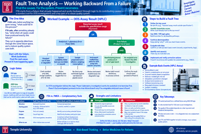
FTA starts from a failure that already happened and works backward through AND/OR logic to its contributing causes — the standard tool for an OOS root-cause investigation, and the mirror image of FMEA’s forward-looking approach.
The one idea
FMEA asks, before anything has gone wrong, “what could fail in this process?” FTA asks, after something already has, “what chain of causes could have produced exactly this failure?” They run in opposite directions through the same failure space, and a mature quality system uses both.
Mechanics
A fault tree starts with a single, precisely defined top event — the failure that occurred — and branches downward through logic gates to the conditions that could produce it:
An AND gate means every branch beneath it must be true for the event above to occur (e.g., a wrong result reaches release and the reviewer misses it).
An OR gate means any one branch beneath it is sufficient (e.g., a degraded standard, a mis-set instrument parameter, or a transcription error could each independently cause a wrong reported value).
The tree bottoms out in basic events — causes you either confirm or rule out with data, not further decomposition. No formal Boolean notation is required to use this at the bench; the value is in the discipline of writing every “or this could have happened” branch down before deciding which one is true.
Worked example — an out-of-specification (OOS) assay result
Top event: Reported assay result outside the specification range.
Reported assay OOS
 └─ OR: Result is a true failure vs. a lab/analytical error
     ├─ OR (analytical/lab error branch)
     │    ├─ Standard was out of date or degraded
     │    │    → check standard prep date, storage conditions, prior QC data
     │    ├─ System suitability failed but was overridden or missed
     │    │    → review the suitability data logged that run
     │    ├─ Sample preparation error (dilution, weighing, transcription)
     │    │    → re-check the prep worksheet against the raw balance/pipette record
     │    └─ Instrument malfunction (detector drift, pump seal, injector carryover)
     │         → review instrument maintenance and diagnostic logs
     └─ AND (true-failure branch)
          ├─ Manufacturing process produced an out-of-spec batch
          │    → review batch record deviations, in-process controls
          └─ No analytical error found in the OOS investigation above
               → confirms the result should stand
An OOS investigation under Q7/GMP follows exactly this shape: Phase I (laboratory investigation) works the analytical-error branches first, because a confirmed lab error can invalidate the result without ever reaching the manufacturing branch; Phase II (full investigation) only proceeds down the true-failure branch once Phase I finds no assignable analytical cause.
When to reach for it vs. FMEA
FTA is reactive — it exists because a specific, already-observed failure needs a root cause, and it only makes sense once that top event is precisely defined. FMEA is prospective — it exists to find failure modes before they happen, and it doesn’t require anything to have gone wrong yet. In practice, a documented FMEA is often what an OOS investigation checks against: “was this failure mode already identified, and if so, why did the existing control not catch it?”
Known weaknesses
FTA is only as good as the top event’s definition — a vaguely stated failure (“something went wrong with the assay”) produces an unusably broad tree.
Trees for a complex, multi-step method can become large fast; without discipline about what counts as a “basic event,” the tree can sprawl without converging on an actionable root cause.
FTA doesn’t score or prioritize the way RPN does — it’s a diagnostic tool for one failure, not a ranking tool across many, which is why it’s typically paired with an FMEA or risk ranking rather than used as the whole risk program.
2.3 - HACCP — Critical Control Points, Borrowed From Food Safety
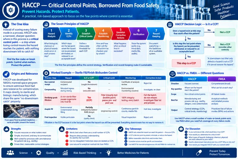
Hazard Analysis and Critical Control Points asks a narrower question than FMEA: not every failure mode in a process, but where the few points are whose failure directly threatens the patient — worked through a sterile-fill bioburden-control example.
The one idea
Instead of scoring every failure mode in a process, HACCP asks a narrower, sharper question: where in this process is a critical control point — a step where losing control means the hazard reaches the patient, with nothing downstream left to catch it?
Mechanics
HACCP originated in food safety (developed for NASA’s manned space program, to guarantee astronaut food had zero tolerance for contamination) and maps cleanly onto sterile and biologic manufacturing, which share that same “no downstream catch” property. The full method has seven principles; the ones that matter for a control-strategy discussion are:
Conduct a hazard analysis — what biological, chemical, or physical hazards could occur at each process step?
Identify critical control points (CCPs) — of all the steps, which ones are the point where the hazard can still be prevented, eliminated, or reduced to an acceptable level? A step downstream of the true control point is not itself a CCP, even if a hazard could theoretically show up there.
Establish critical limits — a measurable threshold for each CCP (a temperature, a pressure differential, a bioburden count) that separates “in control” from “out of control.”
Establish monitoring — how and how often the critical limit is checked, and by whom.
Establish corrective action — what happens, specifically, the moment a critical limit is exceeded.
(The remaining two principles — verification and record-keeping — are the documentation backbone that makes the first five auditable, and aren’t specific to any one CCP.)
Worked example — sterile fill/finish bioburden control
Step
Hazard
Is it a CCP?
Critical limit
Monitoring
Corrective action
Raw material receipt
Contaminated excipient
No — caught downstream
—
Certificate of analysis review
Reject lot
Compounding
Microbial ingress during mixing
No — bioburden reducible later
—
Environmental monitoring (routine)
Investigate, re-clean
Sterilizing-grade filtration
A non-sterile filter passes organisms into the final fill
Yes — nothing downstream removes a missed organism
Filter integrity test (bubble point) passes pre- and post-use
100% integrity testing, every batch
Fail the batch; do not release; investigate filter lot and process
Aseptic fill
Environmental contamination during filling
Partially — mitigated by isolator/RABS design, not a single measurable limit
— (engineering control, not a CCP in the classic sense)
Continuous particle counts, media fills
Halt line, investigate
Final inspection
Visible particulate
No — a quality check, not a hazard-elimination point
—
Visual inspection
Reject unit
The filtration step is the CCP because it is the last point where the hazard (a non-sterile product) can still be prevented — everything upstream can be caught or corrected later in the process, and everything downstream has no way to remove an organism that already got through. That is the test for “is this a CCP,” not “could something go wrong here.”
When to reach for it vs. FMEA
FMEA decomposes an entire process into every failure mode and scores each one — useful when you want comprehensive coverage of a method or process. HACCP deliberately does the opposite: it narrows attention to the small number of points where losing control is unrecoverable, which is exactly right for manufacturing and process risk (sterility assurance, allergen control, cross-contamination) but a poor fit for analytical method risk, where FMEA’s step-by-step, fully-scored decomposition is what regulators and most labs actually expect.
Known weaknesses
Works best when there really are a small number of make-or-break points; forcing a HACCP structure onto a process with many, roughly-equally-important risks just reproduces an FMEA with extra steps.
Identifying the true CCP takes real process understanding — misidentifying a downstream inspection point as a CCP gives false confidence, since it doesn’t actually prevent the hazard, only detects it after the fact.
Less natural for analytical-method risk (where FMEA dominates) than for manufacturing/process risk, where it originated and still fits best.
2.4 - HAZOP — Deviations From Design Intent
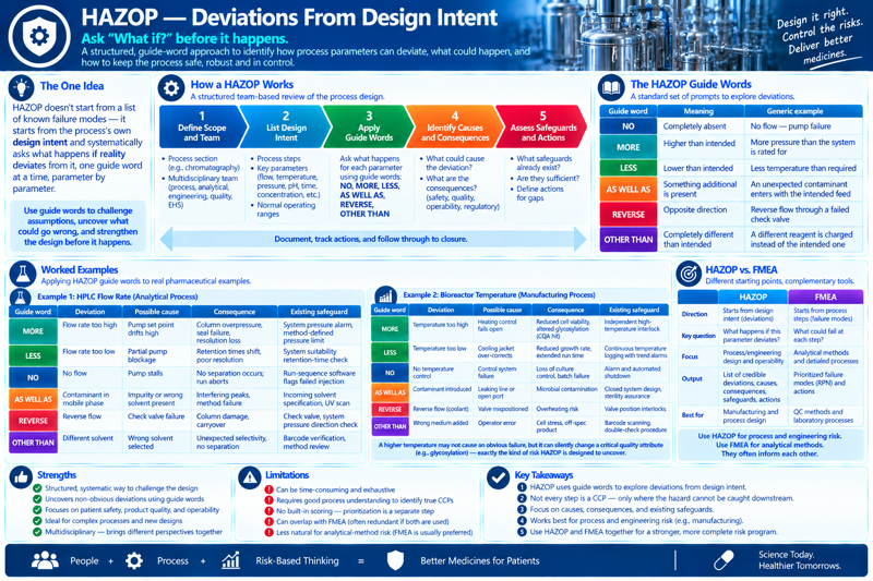
Hazard and Operability study asks, guided word by guided word, what happens if a process parameter is too much, too little, reversed, or accompanied by something unintended — a process/engineering tool applied here to a chromatography example.
The one idea
HAZOP doesn’t start from a list of known failure modes the way FMEA does — it starts from the process’s own design intent and systematically asks what happens if reality deviates from it, one guide word at a time, parameter by parameter.
Mechanics
For each parameter at each step of a process (flow rate, temperature, pressure, pH, concentration, time), a HAZOP team applies a fixed set of guide words and asks what a deviation of that kind would actually cause:
Guide word
Meaning
Generic example
NO
The parameter is completely absent
No flow — pump failure
MORE
The parameter is higher than intended
More pressure than the system is rated for
LESS
The parameter is lower than intended
Less temperature than the reaction requires
AS WELL AS
Something additional is present
An unexpected contaminant enters with the intended feed
REVERSE
The parameter or flow runs backward
Reverse flow through a check valve that has failed
OTHER THAN
Something completely different happens instead
A different reagent is charged than intended
Unlike FMEA, HAZOP doesn’t score every deviation on Severity/Occurrence/Detection — the output is a qualitative list of credible deviations, their causes, consequences, and existing safeguards, with follow-up actions where the safeguards look thin.
Worked example — HPLC flow rate and a bioreactor’s temperature
Guide word
Parameter
Deviation
Consequence
Safeguard
MORE
HPLC flow rate
Pump set point drifts high
Column overpressure, potential seal failure, resolution loss
System pressure alarm, method-defined pressure limit
LESS
HPLC flow rate
Partial pump blockage
Retention times shift, poor resolution between API and impurity
System suitability retention-time check
NO
HPLC flow rate
Pump stalls
No separation occurs at all; run aborts
Run-sequence software flags a failed injection
MORE
Bioreactor temperature
Heating control fails open
Reduced cell viability, altered glycosylation profile (a CQA hit)
Independent high-temperature interlock, separate from the control loop
LESS
Bioreactor temperature
Cooling jacket over-corrects
Reduced growth rate, extended run time
Continuous temperature logging with trend alarms
Notice the bioreactor row: a MORE temperature deviation doesn’t just risk an obvious failure (dead cells) — it can silently shift a critical quality attribute (glycosylation) while the culture still looks healthy, which is exactly the kind of consequence a guide-word walk-through is designed to surface deliberately, rather than relying on someone to have already thought of it.
When to reach for it vs. FMEA
HAZOP and FMEA overlap heavily in outcome — both end up identifying deviations and their consequences — but HAZOP is organized around the process’s design intent, parameter by parameter, which makes it a natural fit for engineering and process-design teams examining a new unit operation (a reactor, a filtration skid, a chromatography skid) before it’s ever run. Most QC labs default to FMEA for method risk because the “steps” of a method are already well defined; HAZOP earns its keep more in process/engineering contexts where the parameters, not discrete process steps, are the natural unit of analysis.
Known weaknesses
Applying every guide word to every parameter at every step can be slow and exhaustive for a complex process — teams often scope it to the parameters most likely to matter, which reintroduces some of the same judgment calls HAZOP is meant to avoid.
Without a scoring step, prioritizing which deviations to act on first is a separate, later exercise — HAZOP tells you what could deviate, not which deviation matters most.
The overlap with FMEA means running both on the same process is often redundant; most sites pick one as the primary tool for a given risk type (HAZOP for process design, FMEA for methods) rather than running both routinely.
2.5 - Risk Ranking and Filtering — Comparing Risks That Don't Share a Scale
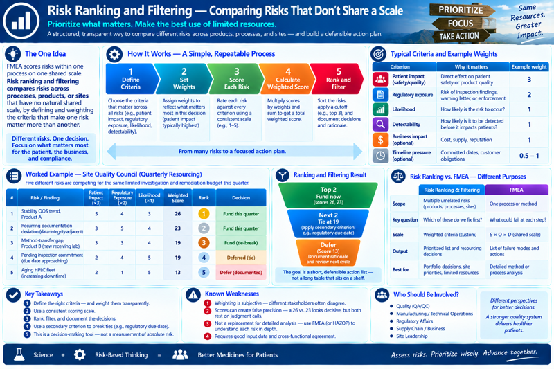
When risks come from different processes, products, or sites and don’t share a common scale, risk ranking and filtering normalizes them against weighted criteria to build one prioritized list — worked through a site quality council’s quarterly resourcing decision.
The one idea
FMEA scores risks within one process on one shared scale. Risk ranking and filtering compares risks across processes, products, or sites that have no natural shared scale at all, by explicitly defining and weighting the criteria that make one risk matter more than another.
Mechanics
Define criteria that matter across every risk being compared — typically patient impact, regulatory exposure, likelihood, and detectability, though a portfolio-level exercise might add business impact or timeline pressure.
Weight the criteria to reflect what actually matters most in this decision (patient impact usually carries the most weight; timeline pressure usually carries the least, if it’s included at all).
Score each risk against every criterion, using whatever scale is practical (often 1–5, sometimes qualitative bands converted to numbers).
Compute a weighted score and rank — then filter: set a threshold or a headcount/budget cutoff and act on what clears it, explicitly documenting why anything below the line is being deferred.
The “filtering” half is as important as the ranking half — the exercise exists to produce a short, defensible action list, not just a long sorted table nobody acts on.
Worked example — a site quality council’s quarterly resourcing decision
Five unrelated findings are competing for the same limited investigation and remediation budget this quarter:
Risk
Patient impact (×3)
Regulatory exposure (×2)
Likelihood (×1)
Weighted score
Stability OOS trend, Product A
5
4
3
5×3 + 4×2 + 3×1 = 26
Method-transfer gap, Product B (new receiving lab)
Pending inspection commitment (due date approaching)
2
4
5
2×3 + 4×2 + 5×1 = 19
Ranked and filtered against a “fund the top three this quarter” cutoff: the stability OOS trend (26) and the documentation deviation (23) fund first regardless of tiebreaks; the method-transfer gap and the inspection commitment tie at 19 and need a secondary criterion (e.g., regulatory due date) to break the tie for the third slot. The aging-fleet risk (13) is explicitly deferred — not ignored, documented as deferred, with the reasoning on record for the next review cycle.
When to reach for it vs. FMEA
Use risk ranking and filtering when the decision spans multiple unrelated risks competing for the same finite resource — funding, staffing, audit time — not when you’re working through the failure modes of a single process or method, which is FMEA’s job. It’s the tool for “which of these five different problems do we fix first,” not “what could go wrong in this one method.”
Known weaknesses
The weighting scheme is itself a subjective judgment call — this is the same criticism Q9(R1) raises about FMEA’s Severity/Occurrence/Detection scoring; risk ranking and filtering doesn’t remove that subjectivity, it just moves it up a level, from scoring individual failure modes to weighting the criteria that compare them.
Different stakeholders (quality, manufacturing, regulatory affairs) often disagree on the weights themselves — reaching agreement on the weighting is frequently the harder part of the exercise, not the scoring.
A weighted score can create false precision — a 26 vs. a 23 looks decisive, but both numbers rest on the same soft inputs as any other risk score, and the ranking should be sanity-checked qualitatively before being treated as a tiebreaker.
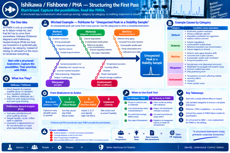
2.6 - Ishikawa / Fishbone / PHA — Structuring the First Pass
Before an FMEA can score failure modes, it needs a reasonably complete list of them — fishbone diagrams and Preliminary Hazard Analysis are how that list gets brainstormed systematically, worked through an unexpected-peak example that feeds directly into an FMEA.
The one idea
An FMEA is only as complete as its failure-mode list, and that list has to come from somewhere. Ishikawa (fishbone) diagrams and Preliminary Hazard Analysis are how you brainstorm it systematically, category by category, instead of relying on whoever’s in the room to remember everything from experience.
Mechanics
An Ishikawa diagram starts from a defined effect (an observed or feared problem) and branches into standard categories of contributing cause. Adapted for an analytical lab, the categories are usually:
Method — the procedure itself: parameters, steps, order of operations
Environment — temperature, humidity, lighting, vibration, power quality
Preliminary Hazard Analysis (PHA) is a lighter, earlier-stage cousin — a first-pass brainstorm of what could possibly go wrong before a process even exists in detail, often just a simple hazard/cause/effect table, used to scope what a later, more formal risk assessment needs to cover.
Worked example — “unexpected peak in a stability sample”
Category
Candidate causes brainstormed
Method
Insufficient gradient resolution; wrong wavelength selected; integration parameters too aggressive
Materials
Column degradation; contaminated mobile phase; reference standard cross-contamination
Machine
Detector lamp aging (baseline drift creating false peaks); carryover from a prior injection; autosampler needle wash insufficient
Manpower
Sample prep error introducing a degradant precursor; mislabeled vial swapped with another study
Environment
Lab temperature excursion affecting sample stability between prep and injection
This is deliberately a long, unfiltered list — the point of the fishbone pass is coverage, not judgment. Three or four of these branches then become the failure-mode column of a follow-on FMEA: “contaminated mobile phase” becomes a scoreable failure mode with its own severity, occurrence, and detection; “detector lamp aging” becomes another. The fishbone did the brainstorming; the FMEA does the prioritizing.
When to reach for it vs. FMEA directly
Skip straight to FMEA when the failure modes are already well understood from experience — a mature, well-characterized method rarely needs a fresh fishbone pass. Reach for Ishikawa or PHA first when the process or method is new or unfamiliar, or when a cross-functional team is starting from very different mental models of what could go wrong and needs a shared, structured brainstorm before anyone starts scoring anything.
Known weaknesses
Purely qualitative — a fishbone diagram or PHA table has no scoring or prioritization built in; it can surface a long list of contributing factors without telling you which ones actually matter.
Coverage depends heavily on who’s in the room; the category headings help structure the brainstorm, but they don’t guarantee completeness the way a systematic top-down decomposition (like FMEA’s step-by-step structure) does.
It is not, on its own, a complete quality risk management record — it’s the front end that typically feeds into an FMEA or risk ranking and filtering exercise, not a substitute for either.