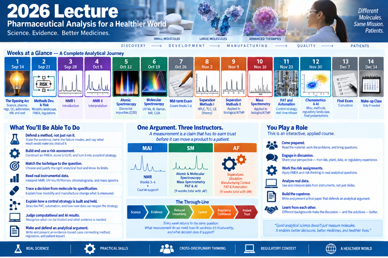
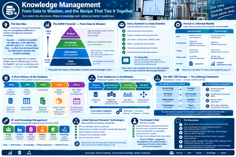
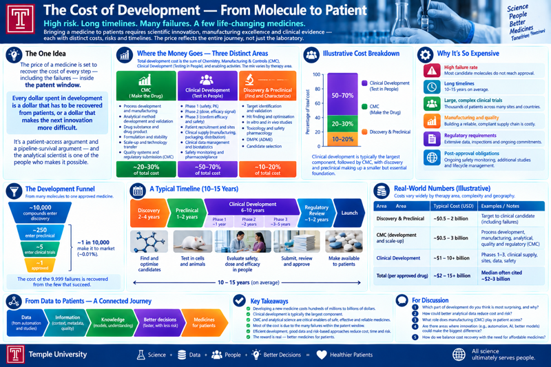
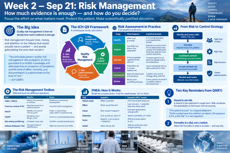
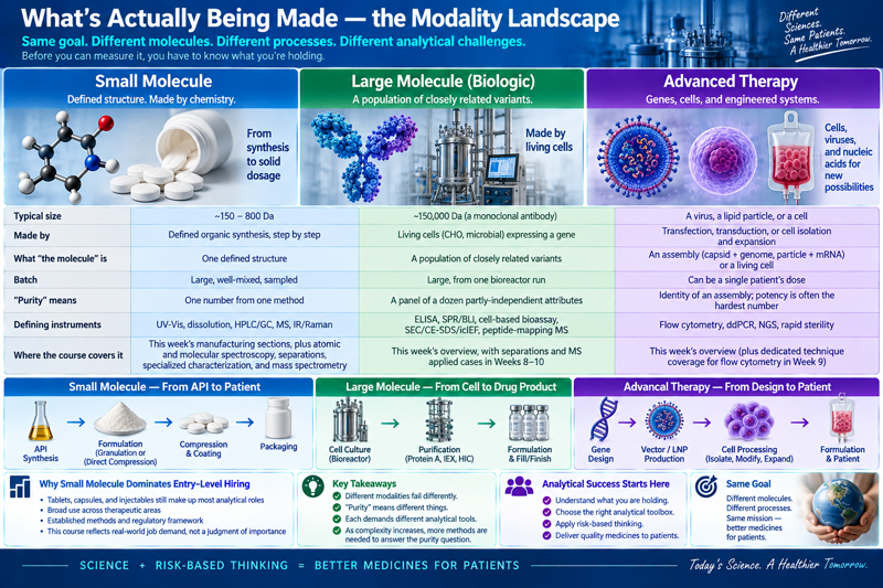
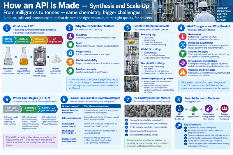
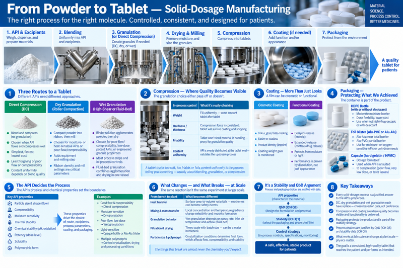
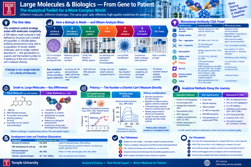
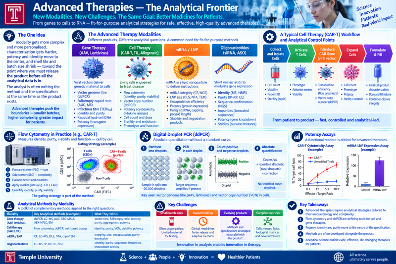
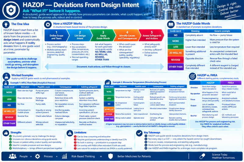
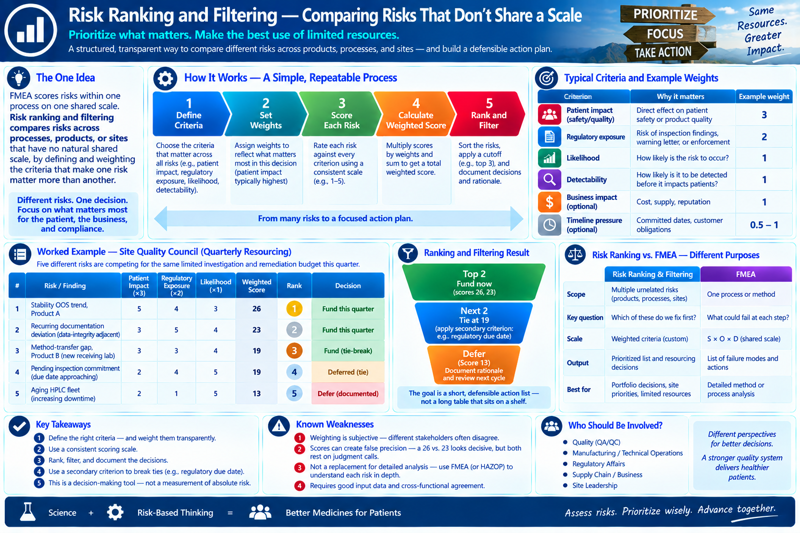
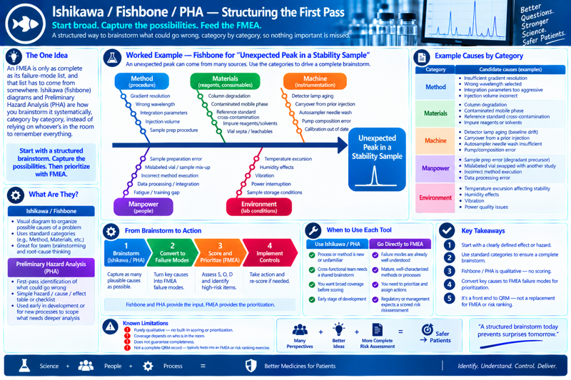
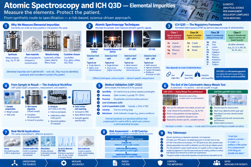
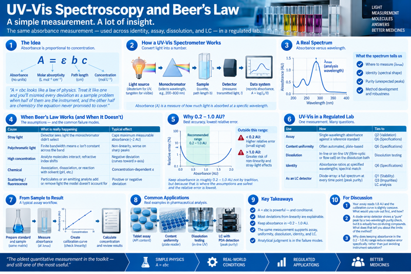
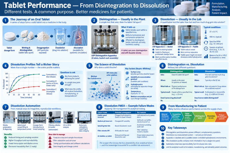
The 2026 course, week by week, aligned to the real syllabus and its three instructors (MAI, SM, AF). Week 1 opens the arc; Week 2 covers methods development, the modality landscape, and risk; Weeks 3–4 are NMR (MAI); Weeks 5–6, 8–10 teach each technique AF and SM lead in turn; Week 11 is PAT and automation; Week 12 is chemometrics, miscellaneous methods, and final papers — bracketed by the mid-term and the final exam.
This is the 2026 course, organised weeek by week to match the department’s actual syllabus. Each week has its own folder in the left menu.
What you’ll be able to do
By the end of the term, you should be able to:
Defend a method, not just run it. For any validated analytical method, state what evidence supports it, name its most likely failure modes, and say what result would make you distrust it.
Build and use a risk assessment. Construct a method or process FMEA, score severity, occurrence, and detection without inflating detection to look reassuring, and turn the assessment into a control strategy a regulator could follow (Week 2, and the risk-homework checkpoints in Weeks 5, 6, and 10).
Match the technique to the question. Given an analytical problem — an elemental impurity, an unknown degradant, a charge-variant shift, a polymorph question — choose and justify the right technique among NMR, atomic and molecular spectroscopy, chromatography, solid-state/thermal characterization, flow cytometry, and mass spectrometry, and state what that technique can’t tell you (Weeks 3–10).
Read real instrumental data. Interpret an NMR spectrum, a UV-Vis/IR/Raman trace, a chromatogram, or a mass spectrum well enough to identify a structure, flag a co-elution or ion-suppression artifact, or catch a spectral match that looks right but isn’t.
Trace a decision from molecule to specification. Explain how what’s being made — small molecule, biologic, or advanced therapy — changes which failure modes matter and how “identity” or “purity” is even defined, and read a Certificate of Analysis line by line back to the method and manufacturing step behind it.
Explain how a control strategy is built, held, and reopened. Describe the at-/on-/in-line measurement hierarchy and real-time release testing, and how a complaint or pharmacovigilance signal can force a control strategy that passed every existing test to be revisited (Week 11).
Judge whether a computational or AI-based result can be trusted. Distinguish predictive/chemometric models from generative AI by how each is governed, recognise information leakage or an out-of-domain prediction, and state what evidence a model needs before it can support a regulatory decision (Week 12).
Make and defend an evidence-based analytical argument in writing, naming a method’s failure modes and their detectability and connecting the technique to a regulatory expectation and a patient consequence (final paper and capstone).
One argument, taught by three instructors
The course is not a tour of instruments. It is a single argument — a measurement is a claim that has to earn trust before it can move a product or a patient — and it’s taught by three people: MAI, SM, and AF. AF and SM together lead nine of the term’s lecture sessions; MAI leads two (NMR); the rest are the mid-term, the final, and the occasional make-up.
NMR (Weeks 3–4, MAI). Introduction to NMR spectroscopy, then interpretation — the one part of the term AF and SM hand off entirely.
The AF/SM technique arc (Weeks 5–6, 8–10). Atomic spectroscopy and molecular spectroscopy (with UV-Vis and a Certificate-of-Analysis read-through) are taught on the small molecule alone; separation methods and mass spectrometry each add an applied case extending the same technique to biologics and advanced therapies. In between, Week 9 pivots to the specialized and solid-state techniques that don’t fit that main arc but are load-bearing in a real QC lab — DSC/TGA, X-ray powder diffraction and crystallography, flow cytometry, and dissolution. A risk-homework thread runs through the atomic-spectroscopy, molecular-spectroscopy, and mass-spectrometry weeks.
The mid-term falls after the first technique pair; the final is cumulative, with Week 14 held only if a make-up session is absolutely necessary. Every week returns to the same refrain: science → evidence → reduced uncertainty → control → regulatory confidence → patient trust.
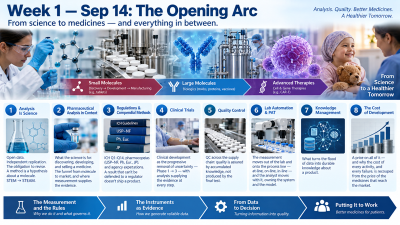
Week 1 — Sep 14 is the opening arc in full, and it is substantial: it moves deliberately in one direction — science → pharma → regs — then reframes clinical development as the progressive removal of uncertainty and turns to the working detail: quality control across the supply chain, lab automation and process analytical technology, knowledge management, and the cost of development. It is the whole course in miniature; the weeks that follow slow down and do the work.
Work through each week’s sections in order; use the “On this page” list on the right to move within a section, and the ← / → buttons at the foot of each page to step through the course in sequence.
1 - Week 1 — Sep 14: The Opening Arc
Lecture 1 in full: from what makes analysis a science, to what that science is for inside a company that discovers, develops, and sells medicines, to the regulations that govern every analytical decision — and on to quality control, automation, knowledge management, and cost.
Everything in this folder is Lecture 1. It is the opening arc of the course, and it moves deliberately in one direction — science → pharma → regs — before turning to the working detail that fills the rest of the term.
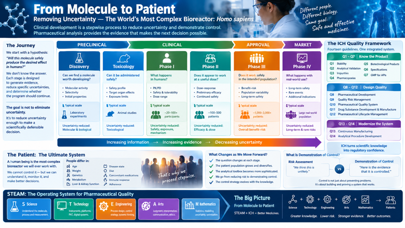
It also plants the course’s three movements in one sitting: the measurement and the rules (sections 1–3), the modalities, made and measured together (sections 4–6, and the three-modality arrow above — small molecule, large molecule, advanced therapy, each taught with the instruments that characterise it), and from data to decision (section 7). Later weeks slow each of these down.
Pharmaceutical analysis meets the full definition of science: open data, independent replication, and the obligation to revise. A method is a hypothesis about a molecule. STEM → STEAM — the “A” (judgment, interpretation, design, communication, ethics) is what separates an analyst from a technician.
What that science is for: discovering, developing, and selling a medicine. The funnel from molecule to market, and where measurement supplies the evidence at each narrowing.
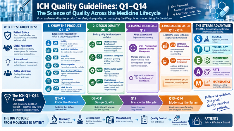
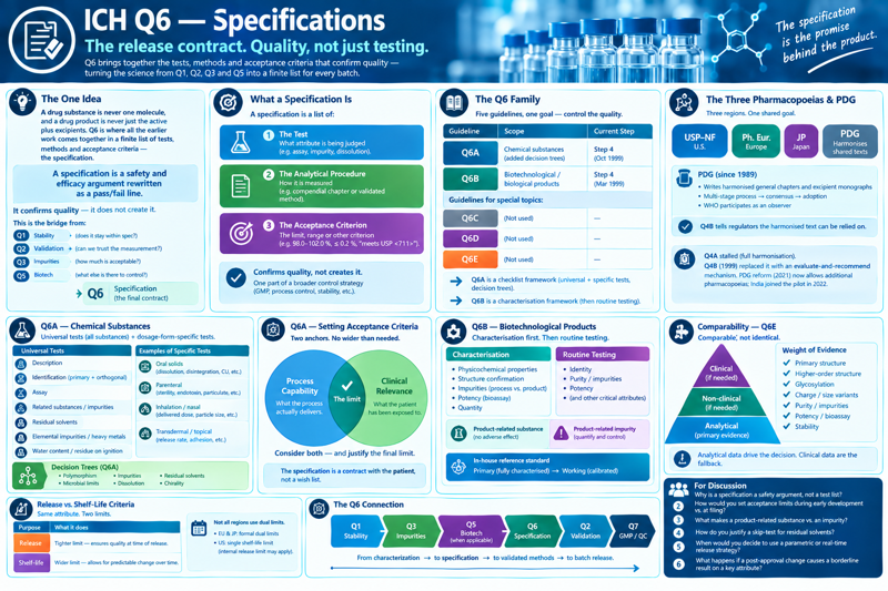
The regs end of the funnel — the ICH quality guidelines (Q1–Q14), the pharmacopeias (USP–NF, Ph. Eur., JP), and agency expectations. A result that can’t be defended to a regulator doesn’t ship a product. Includes a full page on each ICH quality guideline that touches analysis, from Q1 · Stability through Q14 · Analytical QbD.
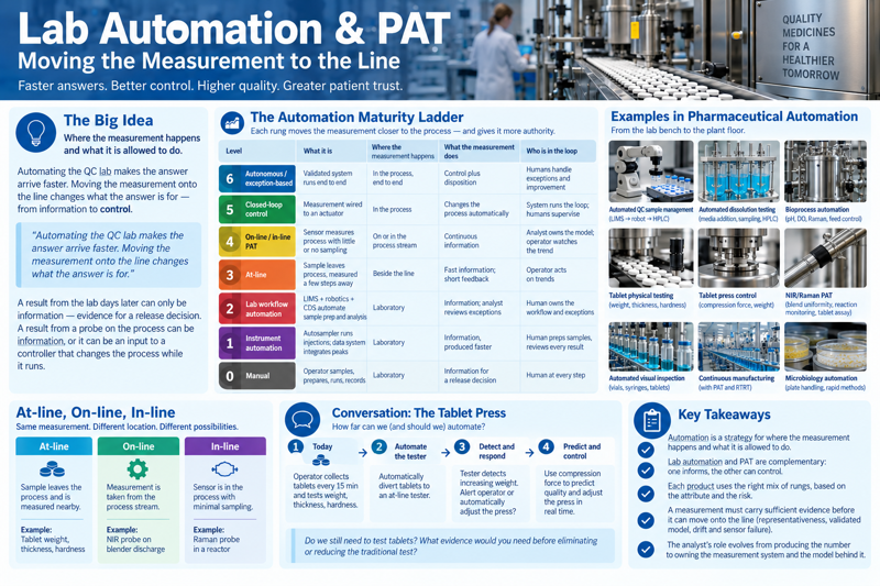
The measurement moves out of the laboratory and onto the process line — at-line, on-line, in-line — and the analyst moves with it, owning the system and the model rather than the number.
A price on all of it — and why the cost of every activity, and every failure, is recouped from the price of the medicines that reach the market.
How to use this
Work through the sections in order. Use the menu on the left to see where you are, the “On this page” list on the right to move within a section, and the ← / → buttons at the foot of each page to step through the whole lecture in sequence.
Later weeks each get their own folder in the left menu.
On the job
This course is built around a simple test: could you use this in your first month in an analytical role? A few things that are true on day one, regardless of company or modality:
Every result you generate is a GMP record the moment it’s written down — dated, signed, and defensible, not a scratch-pad number.
You will spend far more time reading and defending other people’s results (a CoA, a stability report, an OOS investigation) than generating your own from a blank page.
“The SOP says so” is not a reason a regulator accepts — you will be asked why the SOP says so, and the answer is always evidence and risk.
Nobody will hand you a finished specification. You will be handed a partial one and asked whether it’s still adequate — which is exactly what Week 2 starts teaching you to judge.
1.1 - Pharmaceutical Analysis Is Science — From STEM to STEAM
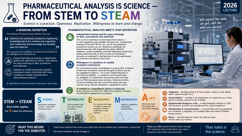
The opening frame for the 2026 course: why pharmaceutical analysis is a science in the full sense of the word, and what the ‘A’ in STEAM adds to it.
Every year this course opens with a question that sounds settled but isn’t: is what we do a science, or is it just a set of techniques we run? Your answer shapes how you’ll spend the rest of the term — and, frankly, your career.
A working definition
The American Physical Society defines it this way:
Science is the systematic enterprise of gathering knowledge about the universe and organizing and condensing that knowledge into testable laws and theories.
The success and credibility of science are anchored in the willingness of scientists to:
Expose their ideas and results to independent testing and replication by others. This requires the open exchange of data, procedures and materials.
Abandon or modify previously accepted conclusions when confronted with more complete or reliable experimental or observational evidence.
I like this definition because it doesn’t lead with test tubes or equations. It leads with a set of commitments — to openness, to replication, and to changing your mind. That is a definition built around continuous learning.
Pharmaceutical analysis meets that definition
Hold our field up against those two commitments and it lines up point for point.
Independent testing and the open exchange of data, procedures and materials. This is not an aspiration in pharmaceutical analysis — it is the regulatory and scientific infrastructure. Compendial methods in the USP–NF, Ph. Eur. and JP are published procedures anyone can run. Reference standards are shared materials with characterized values. Method validation, system suitability, and inter-laboratory proficiency testing exist precisely so that a result is not believed because we produced it, but because it can be reproduced by someone who doesn’t work here.
Willingness to abandon or modify accepted conclusions. An out-of-specification investigation is exactly this: evidence arrives that contradicts what we thought we knew, and we are obligated to follow it. So is the method lifecycle in ICH Q14 and Q2(R2) — a method is not finished when it’s validated; it is monitored, and revised when the data say so. Pharmacopeias issue revisions. Guidance evolves. A control strategy that was current five years ago may now be wrong, and the discipline is designed to notice.
A method, in this light, is a hypothesis about a molecule. Every injection is a test of it. When the system suitability fails, when the recovery drifts, when a new impurity appears — the discipline doesn’t ask us to defend the old conclusion. It asks us to update it.
STEM → STEAM
We usually file analytical chemistry under STEM, and each letter genuinely applies:
Science — the reasoning above: hypothesis, evidence, revision.
Technology — the instruments: LC, GC, mass spec, NMR, spectroscopy.
Engineering — the systems that make a number trustworthy: sampling plans, control strategies, qualification, data integrity.
But the letter that’s usually left out is the one that separates a technician from an analyst. The A — Arts — is not decoration:
Judgment — deciding what is fit for purpose, what is a real signal, when “close enough” isn’t.
Interpretation — reading a chromatogram or a spectrum as a story about a sample, not just a set of peaks.
Experimental design as craft — a well-designed method or DOE has the same economy as a good proof or a good sentence.
Visualization and communication — a result that can’t be explained to a reviewer, a regulator, or a patient advocate hasn’t finished being science.
Ethics — the discipline to report the data you got, not the data you wanted.
STEM gives you the tools. The A is what you bring to them.
What this means for the semester
Treat every method we cover as a claim that can be tested and, sometimes, overturned. Ask what evidence would change it. Keep your data and procedures open enough that someone else could check your work — because in this field, someone will. That habit is the science.
1.2 - Pharmaceutical Analysis in a Regulated Organization
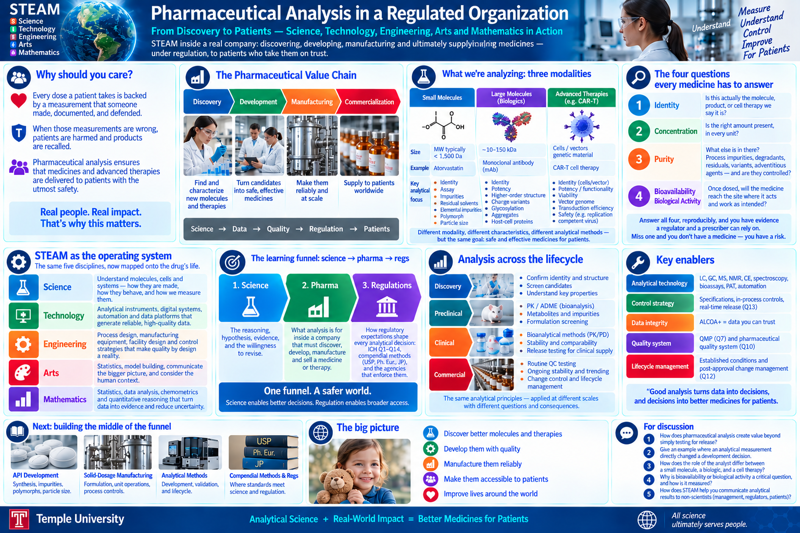
What STEM-to-STEAM looks like once it’s inside a company that has to discover, develop, and ultimately sell a novel medicine — and the science → pharma → regs funnel this course follows.
The last section argued that pharmaceutical analysis is science: hypothesis, evidence, and the willingness to revise. Now the setting changes. Put that science inside an organization whose job is to discover a molecule, develop it into a medicine, and ultimately sell it — under regulation, to patients who will take it on trust. STEAM doesn’t get left at the lab door. It becomes the operating system of the whole company.
Why should you care?
Pharmaceutical analysis is the set of practices used to ensure that medicines and devices are delivered to patients with the utmost safety. Every dose a patient takes is backed by a measurement that someone made, documented, and defended. When those measurements are wrong, patients are harmed and products are recalled. That is the stake behind everything in this course.
What we’re analyzing: the API
We will focus on the Active Pharmaceutical Ingredient (API) — the component that does the therapeutic work. APIs fall into two broad classes, and they demand different analytical toolboxes:
Small molecule
Large molecule
Size
MW below ~1,500 Da
Proteins, monoclonal antibodies — tens of kDa and up
Structure
Defined, drawable
Folded, heterogeneous, sensitive to its environment
Typical methods
HPLC/UHPLC, GC, LC–MS, NMR, dissolution
Peptide mapping, CE, SEC, icIEF, LC–MS of intact and reduced forms, potency bioassays
Different molecule, different instruments — but the same four questions.
The four questions every medicine has to answer
Leveraging state-of-the-art analytical technology, the medicine is characterized to establish:
Identity — is this actually the molecule we say it is?
Concentration (strength / assay) — is the right amount present, in every unit?
Purity — what else is in there? Process impurities, degradation products, residual solvents, and — for large molecules — aggregates and variants.
Bioavailability — once dosed, will the API actually reach the site where it acts?
Answer all four, reproducibly, and you have evidence a regulator and a prescriber can rely on. Miss one and you don’t have a medicine — you have a compound.
STEAM as the operating system of a regulated company
The same five letters from Lecture 1, now mapped onto the drug’s life:
Science — during discovery, characterization tells you whether you even have the molecule you intended, and how it behaves.
Technology — during development, the analytical platform (LC, MS, NMR, spectroscopy, bioassay) generates the data that defines the product.
Engineering — the control strategy: specifications, sampling plans, in-process controls, method qualification, and data integrity — the systems that make a number trustworthy at commercial scale.
Mathematics — statistics, calibration, uncertainty, stability modeling, and the setting of acceptance criteria that are neither too loose to be safe nor too tight to be manufacturable.
Arts — the judgment to decide what is fit for purpose at each stage, to interpret a result in context, and to explain it to a reviewer, an inspector, or a patient advocate.
The learning funnel: science → pharma → regs
This course moves in that order on purpose:
Science — the reasoning. (Lecture 1.)
Pharma — this section: what analysis is for inside a company that must discover, develop, and sell a medicine.
Regs — how regulatory expectation shapes every analytical decision: the ICH guidelines (Q1–Q14), general compendial methods (USP–NF, Ph. Eur., JP), and the agencies that enforce them. We’ll get into ICH in detail later; for now, just know that the analytical work has to follow it.
The sections that follow build out the middle of that funnel:
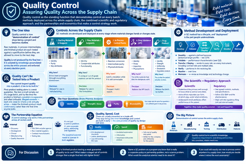
Quality Control (QC) — the function that tests material against its specification and releases (or rejects) it.
Physical and chemical properties of drug molecules — solubility, pKa, partition, polymorphism, and stability, and why each one drives an analytical or formulation decision.
General compendial methods and the regulatory influence on analytical development — where the “standard” methods come from, and how regulatory expectation pulls method development in a particular direction from day one.
1.3 - Regulations & Compendial Methods
The ‘regs’ end of the funnel: how ICH guidelines, the pharmacopeias, and agency expectations shape every analytical decision — from method design to release.
Where this fits
Section 1 established that analysis is science. Section 2 put that science inside a company that has to discover, develop, and sell a medicine. This section is the third step of the funnel — regs — and the through-line is simple: an analytical result that can’t be defended to a regulator doesn’t ship a product.
The ICH framework
What ICH is — the International Council for Harmonisation of Technical Requirements for Pharmaceuticals for Human Use; who its members and observers are; why harmonisation exists (one dataset, multiple markets).
The Quality (“Q”) guidelines that touch analysis directly get a full page each — listed below and in the left menu:
Q1 · Stability — stability testing; defines which methods must be stability-indicating.
Q2 · Validation — validation of analytical procedures (Q2(R2)).
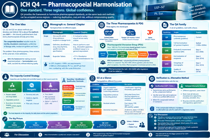
The three major pharmacopeias — USP–NF, Ph. Eur., JP — and how the Pharmacopoeial Discussion Group harmonises chapters across them.
General chapters vs. monographs: a monograph is the spec for a specific article; general chapters are shared methods and policies.
In USP, numbering signals enforceability: chapters below <1000> are requirements, <1000>-and-above are informational.
When you must run the compendial method, and when a validated alternative is allowed (equivalence, and verification under USP <1226>).
How regulation shapes analytical development from day one
Specifications are bounded by ICH limits (Q3A/Q6A) before a method is even developed.
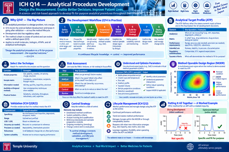
Under Q14 / analytical QbD, the method is designed against its validation targets (Q2(R2)) from the start — an analytical target profile, not a method you validate after the fact.
The stability program (Q1A–F) dictates which methods must exist and what they must resolve.
Data integrity — ALCOA+, audit trails, system suitability as a real-time control — is part of the method, not paperwork around it.
Why you care
Every choice you defended on scientific grounds in Sections 1–2 now has to survive a second audience: an inspector reading your data cold, years later, deciding whether patients can trust it.
1.3.1 - ICH Q1 — Stability Testing
A deep dive into ICH Q1: the purpose of stability testing and the discipline of a systematic program, stress testing versus R&D forced degradation, the chemistry of drug degradation, an integrated forced/accelerated/long-term design, storage conditions, significant change, climatic zones, reduced designs, data evaluation, and the modernized Q1 revision.
The one idea
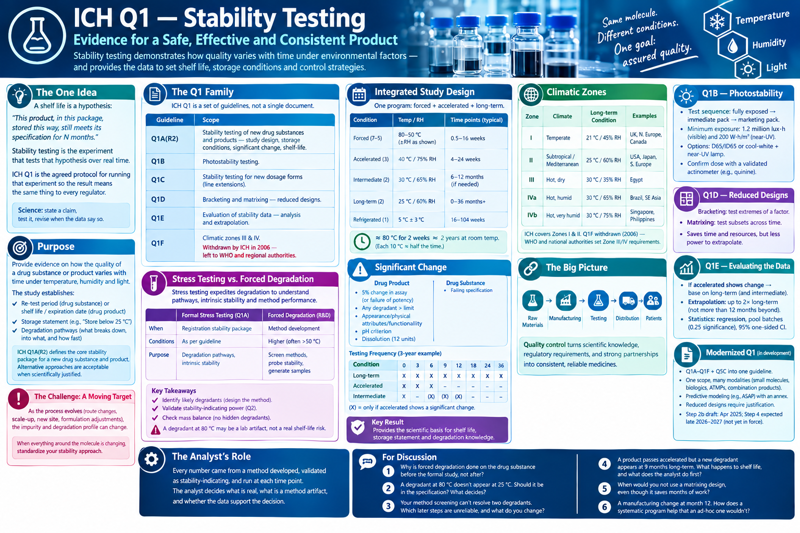
A shelf life is a hypothesis: this product, in this package, stored this way, still meets its specification for N months. Stability testing is the experiment that tests that hypothesis over real time. ICH Q1 is the agreed protocol for running that experiment so that the result means the same thing to every regulator.
This is Lecture 1’s definition of science made concrete — you state a claim, you expose it to testing, and you are obligated to revise the shelf life (or the storage statement, or the formulation) when the data say so.
Purpose
The purpose of stability testing is to provide evidence on how the quality of a drug substance or drug product varies with time under the influence of a variety of environmental factors — temperature, humidity, and light.
From that evidence, and the scientific understanding of the molecule and the product, the study establishes three things:
a re-test period (drug substance) or a shelf life / expiration date (drug product);
the storage statement that goes on the label (“Store below 25 °C”, “Do not refrigerate”, and so on);
the degradation pathways — what breaks down, into what, and how fast.
Q1A defines the core stability package expected for a new drug substance and product. It is a floor, not a straitjacket: alternative approaches are acceptable when they are scientifically justified.
The challenge: a moving target
Here is what makes stability hard in practice. The process by which the drug substance and drug product are made changes as development proceeds — the synthetic route is improved, the scale goes up, the site moves, the formulation is adjusted. Every one of those changes can shift the impurity and degradation profile, which means the “scientific understanding” you were leaning on has to be re-evaluated.
When everything around the molecule is changing, standardize your stability approach.
Fixed conditions, fixed pull points, fixed stability-indicating methods, fixed reporting — the discipline of a systematic program is exactly what lets you compare a batch made this quarter against one made two years ago and actually learn something from the difference.
The Q1 family
ICH Q1 is not one document. It is a set:
Guideline
Scope
Q1A(R2)
Stability testing of new drug substances and products — the core: study design, storage conditions, significant change, shelf-life assignment.
Q1B
Photostability testing.
Q1C
Stability testing for new dosage forms (line extensions of an already-approved product).
Q1D
Bracketing and matrixing — reduced study designs.
Q1E
Evaluation of stability data — how to analyze it and how far you may extrapolate.
Q1F
Stability data for climatic zones III & IV. Withdrawn by ICH in 2006 — left to WHO and regional authorities.
Stress testing and forced degradation
Stress testing is the process of subjecting the drug substance and/or drug product to elevated storage conditions that expedite chemical and physical transformations. The molecule is deliberately degraded with heat, high humidity (75 % RH or greater), acid and base hydrolysis across a pH range, oxidation, and photolysis.
It shows up in two related but distinct activities:
Formal stress testing (ICH Q1A)
Forced degradation in R&D
When
Part of the registration stability package
Early, during method development
Conditions
As outlined in the guideline
Higher — often > 50 °C — for faster answers
Purpose
Establish degradation pathways and intrinsic stability
Screen candidate methods, probe fundamental stability, generate degraded samples
The R&D screening logic is simple: no reaction at the higher temperature → the lower temperatures are very likely fine. Reaction at the higher temperature → confirm it at the formal, “traditional” study conditions before it means anything for the label.
Advantage. Stress testing provides insight into — and a forecast of — the likely degradation products. That helps establish the degradation pathways, the intrinsic stability of the molecule, and, critically, it validates the stability-indicating power of the analytical procedures. The nature of the stress testing depends on the individual drug substance and the type of drug product involved.
Disadvantage. Some chemical and physical transformations observed at higher temperatures do not occur at normal storage conditions, because the activation energies of the processes differ. A degradant that only appears at 80 °C may be a lab artifact, not a shelf-life risk.
For the analyst, the point is not the formal shelf life. The point is to:
Identify the likely degradation products so the method is designed to see them.
Demonstrate the analytical procedure is stability-indicating — it resolves the API from its degradants and can quantify them (ICH Q2 validation depends on this).
Check mass balance — does the loss of assay account for the rise in degradation products? A gap means a degradant you are not detecting.
If you take one thing from Q1 into the lab: forced degradation is how you prove your method can be trusted to watch a product age.
The degradation chemistry
Every extra peak on a stability chromatogram is the product of a chemical reaction. Knowing which reactions a given molecule is prone to tells you what to look for, which conditions accelerate it, and how to build a method that will actually see it. The common routes:
Reaction
What happens
Examples
Hydrolysis
Water cleaves a bond — usually an ester, amide, or lactam. Acid- and base-catalysed, so strongly pH-dependent.
Loss of electrons / gain of oxygen, by three routes: radical autoxidation (trace metals, peroxides, dissolved O₂), photo-oxidation (light, singlet oxygen), and chemical oxidants.
No bonds change — the crystal repacks into a more stable form, altering dissolution and bioavailability.
Ritonavir (1998): a new, more stable form appeared and capsules failed dissolution
Rearrangement. An intramolecular reaction that reorganises the bonding without adding or removing atoms, so the degradant is an isomer of the parent. Because the mass is often unchanged, LC–MS alone will not resolve it from the parent — you need retention, UV spectrum, and sometimes NMR. Acyl glucuronides are a clean example: the acyl group migrates around the sugar ring (1-O → 2-, 3-, 4-O), and the rearranged isomers are the ones that bind covalently to protein.
Decarboxylation. Loss of the carboxyl group as carbon dioxide. It is fast when the carbanion or enol left behind is stabilised — β-keto acids, or aromatic acids with an activating group ortho or para. p-Aminosalicylic acid is the textbook drug example: it decarboxylates to m-aminophenol on mild heating or in solution, which is why PAS discolours on storage.
Dimerization. Two API molecules combine into one covalent species; polymerization is the same reaction run many times. It needs a reactive handle — a β-lactam carbonyl, an aldehyde, an activated alkene, a free thiol. In the aminopenicillins the side-chain amine of one molecule opens the β-lactam of another; the resulting dimers and higher polymers are implicated in penicillin allergy, so they are controlled tightly.
Solution phase vs. solid state. The same molecule degrades differently in the two. In solution it is fully solvated and surrounded by water, so hydrolysis and dissolved-oxygen oxidation dominate and the kinetics are usually clean Arrhenius. In the solid state the molecules are locked in a lattice; reaction happens at surfaces, crystal defects, and amorphous or disordered regions, and is often governed by water sorbed onto the surface rather than bulk water — so rates can be non-Arrhenius and show a moisture threshold. This is why solid-state and solution stress testing are designed and reported separately.
Apparent degradation (recovery). Sometimes the assay comes back low and nothing has actually degraded — the drug has adsorbed onto glass, tubing, or a filter (common for peptides and low-dose products), extraction from the matrix was incomplete, or the reference standard itself has drifted. The check is mass balance again: real degradation shows a matching rise in degradation products; a recovery problem shows a loss with no new peaks. Rule out recovery before you call something degradation.
The degradant-profiling workflow
Forced degradation is not a one-off experiment. It is the first active step in a repeatable, iterative degradant-profiling workflow that runs from what might break all the way to documented structures and mechanisms. One widely cited version (Alsante et al., Adv. Drug Deliv. Rev.59(1), 2007, 29–37) has eight steps:
#
Step
What it involves
Covered in
1
Predict degradants
A degradation database, prediction tools (e.g. CAMEO), and organic-chemistry knowledge
prior knowledge / organic chemistry
2
Design the protocol
A forced-degradation protocol built around the actual chemistry of the API and the drug-product formulation
above
3
Perform the experiments
Stress under reasonable conditions; sample at appropriate points
above
4
Challenge the methodology
HPLC screening of the stressed samples with a suitable screening method
Steps 2–3 are covered above. Steps 4–5 are stability-indicating method development. Steps 6–8 are degradant identification and knowledge capture. And the loop is iterative — a new degradant seen at a later time point, or after a process change, sends you back to step 2 (see The challenge: a moving target).
(Instructor: confirm the citation detail before lecture.)
One program: forced, accelerated, and long-term together
The formal ICH study (the next section) answers the regulator, but on its own it is slow — it is months before it tells the development team whether they are in trouble, and it does not generate degraded material early enough to build methods against. In practice the formal study is run as part of one coordinated program that also spans forced and extra accelerated conditions on a common schedule.
The lever is temperature. As a rule of thumb, a reaction’s rate roughly doubles for every 10 °C (an Arrhenius approximation, Q10 ≈ 2). A marketed formulation is expected to carry about a two-year shelf life, and you cannot wait two years for that answer during development, so higher stressing temperatures stand in for elapsed time. On the doubling rule, ≈ 80 °C for two weeks ≈ two years at room temperature (take room temperature as ≈ 25 °C, the ICH long-term condition):
Stress temperature (°C)
20
30
40
50
60
70
80
Time to a 2-year-equivalent exposure (weeks)
128
64
32
16
8
4
2
Each additional 10 °C halves the time.
A single fast data point is fragile, though, so you set up a gradient of conditions — hot enough for an early read and for method-development samples, mild enough to be relevant, all pulled on one schedule:
Level
Stressing condition
1st pull (wks)
2nd pull
3rd pull
4th pull
7 — forced
80 °C
0.5
1
1.5
2
6 — forced
70 °C
1
2
3
4
5 — forced
60 °C / 75 % RH
2
4
6
8
4 — forced
50 °C
4
8
12
16
3 — accelerated (ICH)
40 °C / 75 % RH
4
8
16
24
2 — long-term (ICH)
25 °C / 60 % RH
16
24
52
104
1 — refrigerated
4 °C
16
24
52
104
One program then gives you two things from the same set of samples: an early read within weeks (are we in trouble?) and the long-term read that supports the filing. The caveat is the disadvantage noted under Stress testing and forced degradation — the forced levels are a screen and a forecast, not the registration answer. Anything they flag is confirmed at ICH conditions before it drives a shelf-life or storage decision.
The formal study design
Batches. At least three primary batches, same synthetic route / manufacturing process, at least pilot scale, in the container closure system proposed for marketing.
Storage conditions (general case):
Study
Condition
Minimum data at submission
Long-term
25 °C ± 2 °C / 60 % RH ± 5 % RH (or) 30 °C ± 2 °C / 65 % RH ± 5 % RH
12 months
Intermediate
30 °C ± 2 °C / 65 % RH ± 5 % RH
6 months
Accelerated
40 °C ± 2 °C / 75 % RH ± 5 % RH
6 months
If 30 °C / 65 % RH is chosen as the long-term condition, there is no separate intermediate condition.
Intended storage
Long-term
Accelerated
Refrigerated
5 °C ± 3 °C
25 °C ± 2 °C / 60 % RH ± 5 % RH
Frozen
−20 °C ± 5 °C
(none — test one batch at ~5 °C or ~25 °C for a comparable period)
Products in semi-permeable containers (e.g. LDPE bags, plastic ampoules) are also tested for water loss at low humidity (40 °C / not more than 25 % RH).
Testing frequency. Long-term: 0, 3, 6, 9, 12, 18, 24 months, then annually through the proposed shelf life. Accelerated: 0, 3, 6 (minimum three points). Intermediate: 0, 6, 9, 12 (minimum four points). A worked schedule for a three-year study, where X is a scheduled pull and (X) is performed only if the accelerated condition shows a significant change:
Condition
0
3
6
9
12
18
24
36
Long-term — 25 °C / 60 % RH
X
X
X
X
X
X
X
X
Accelerated — 40 °C / 75 % RH
X
X
X
Intermediate — 30 °C / 65 % RH
X
(X)
(X)
(X)
“Significant change”
At the accelerated condition, significant change triggers intermediate testing, and the shelf life is then based on long-term data. For a drug product, significant change is any of:
a 5 % change in assay from the initial value (or failure to meet the potency criterion for a biological/immunological method);
any degradation product exceeding its acceptance criterion;
failure to meet acceptance criteria for appearance, physical attributes, or functionality (some physical changes are expected under accelerated stress — e.g. softening of a suppository — and are judged in context);
failure to meet the pH criterion;
failure of dissolution for 12 units.
For a drug substance, significant change is simply failure to meet specification.
Climatic zones and why Q1F was withdrawn
Zone
Climate
Long-term condition
Examples
I
Temperate
21 °C / 45 % RH
UK, Northern Europe, Canada
II
Subtropical / Mediterranean
25 °C / 60 % RH
USA, Japan, Southern Europe
III
Hot, dry
30 °C / 35 % RH
Egypt
IVa
Hot, humid
30 °C / 65 % RH
Brazil, much of SE Asia
IVb
Hot, very humid
30 °C / 75 % RH
Singapore, Philippines
ICH covers Zones I and II. Q1F was withdrawn in 2006 because the ICH regions do not include Zone III/IV countries; WHO and national authorities now set those requirements (WHO recommends 30 °C / 75 % RH long-term for Zone IVb).
Q1B — photostability (in brief)
Test sequence: fully exposed product → immediate pack → marketing pack, stopping once you have enough information. Minimum exposure: 1.2 million lux·hours (visible) and 200 W·h/m² (near-UV). Two lighting options — a D65/ID65 daylight standard (Option 1) or cool-white fluorescent plus a near-UV lamp (Option 2). Light dose is confirmed with a validated actinometer (e.g. quinine).
Q1D — bracketing and matrixing (reduced designs)
Bracketing — test only the extremes of a design factor (strength, container size, fill) at every time point, on the assumption that the extremes bound the intermediates.
Matrixing — test a subset of samples at each time point, a different subset at the next, so the full matrix is covered across the study but not at every pull.
The trade-off — less data means less power to extrapolate. If the data turn out variable, a reduced design may not support the shelf life you wanted, and there is no going back in time.
Q1E — evaluating the data
If accelerated data show significant change, base the shelf life on long-term (and intermediate) data.
Extrapolation — with long-term and accelerated data showing little change and little variability, you may propose a shelf life up to 2× the long-term data period, but not more than 12 months beyond it.
Statistics — regression analysis of each attribute against time; test whether batches can be pooled using analysis of covariance at a 0.25 significance level; the shelf life is the earliest time the 95 % one-sided confidence limit for the mean crosses an acceptance criterion.
Modernization — the revised Q1
ICH is consolidating Q1A–Q1F and Q5C (the biologics stability guideline) into a single modernized Q1 — one unified lifecycle framework (the Step 2b draft runs to roughly 108 pages) that pulls stability testing away from a prescriptive checklist and toward a science- and risk-based strategy, aligned with quality by design and with post-approval lifecycle management (Q12).
The concept paper was endorsed in 2022; the Step 2b draft was released in April 2025, and its public consultation closed late in 2025. Step 4 adoption is anticipated in the late-2026 to 2027 window — so it is not in force yet, but protocols written now will be reviewed under it.
Three shifts matter for how you would design a study:
One scope, many modalities. Rather than guessing which parts of the old series apply to a given product, the new guideline is a common baseline with product-class annexes — synthetic small molecules (including oligonucleotides and peptides), biologics and vaccines (subsuming Q5C), advanced therapy medicinal products (cell and gene therapies), and drug–device combination products.
Predictive modeling gets a regulatory home. A dedicated annex formalizes mathematical and statistical stability modeling — accelerated-assessment approaches such as ASAP that were previously accepted only case by case. Modeled data can be used to justify shelf-life extrapolation and, in some early filings, to stand in for part of the traditional long-term study.
Reduced designs must be earned. Bracketing and matrixing (Q1D) move from protocol templates to a defended position: prior knowledge and platform data, a risk assessment tied to the product and its container closure system, and analytics that show statistically that the reduced matrix will not compromise trend detection.
Because stability studies are multi-year commitments, CMC teams writing protocols today are already auditing their SOPs so they don’t lock legacy assumptions into submissions that will be assessed against the new framework.
(Status as of early 2026 — Step 4 not yet adopted; confirm before lecture.)
Where the analyst sits
Every number in a stability report came from a method an analyst developed, validated as stability-indicating, and ran at each time point — sometimes for years. The judgment calls are analytical: is that a real new peak or a column artifact? Does mass balance close? Is the trend real or within method variability? Q1 is the framework; the analyst is the instrument that makes it mean something.
For discussion
Why is forced degradation done on the drug substance before the formal study, not after?
Forced degradation at 80 °C produces a degradant you never see at 40 °C or 25 °C. Does it belong on the specification? What decides?
A molecule has an ester, a secondary amine, and a stereocentre α to a carbonyl. Which degradation reactions would you screen for first, and which stress condition targets each?
Your method screening (step 4 of the degradant-profiling workflow) can’t resolve two degradants that co-elute. Which later steps are now unreliable, and what do you change?
A product passes accelerated but a new degradant appears at 9 months long-term. What happens to the shelf life, and what does the analyst have to do first?
When would you not use a matrixing design, even though it would save the lab months of work?
The manufacturing process changed at month 12 of a stability study. What does a systematic stability program let you do that an ad-hoc one would not?
1.3.2 - ICH Q2 — Validation of Analytical Procedures
A deep dive into ICH Q2(R2): validation as the demonstration that a measurement is fit for its intended purpose — the analytical procedure as a measurement system, the four procedure types, the analytical figures of merit and their formal definitions (accuracy, precision, specificity, detection and quantitation limits, linearity, range, robustness), which characteristics are required for which test type, the R2 reframing around reportable range and multivariate procedures, stability-indicating methods, platform methods, and validation’s place in the Q14 analytical procedure lifecycle.
The one idea
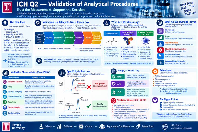
An analytical result is a claim: the assay is 98.7 %, this impurity is at 0.12 %, the API is identified. Validation is the body of evidence that the measurement behind the claim is fit for its intended purpose — accurate enough, specific enough, precise enough, over the range where it is actually used — so that a release or stability decision can rest on it.
This pairs directly with the previous section:
Q1 asks: does the product remain within its specification over time?
Q2 asks: can we trust the analytical evidence used to answer that question?
Without Q2, the conclusions from a stability study are only as good as an unexamined instrument reading. Q2(R2) (Step 4, November 2023; a minor error-correction document followed in 2025) is the current framework, and it was developed alongside Q14 — validation is now explicitly the point in an analytical procedure’s lifecycle where performance is confirmed, not a standalone hurdle.
Validation is not “checking the method”
The naïve mental model is a straight line:
develop method → validate method → use method
Q2(R2), read together with Q14, replaces it with a loop:
Q14 is how you develop a procedure with scientific understanding and risk-based thinking. Q2 is the question:
Can we demonstrate that the resulting procedure performs adequately for the purpose we intend to use it for?
Validation is therefore not the moment science stops. It is a structured demonstration of what is already understood about the measurement system — and relevant data generated during development can contribute to the validation package rather than being repeated.
The challenge: a moving target
The same difficulty that shadows Q1 applies to the method. The synthetic route, the scale, the manufacturing site, and the formulation all change as a function of development time, and each change can shift the impurity and degradation profile the method was built to see. A method validated against last year’s material may need re-validation — to a degree that scales with the size of the change.
When everything around the molecule is changing, standardize your analytical approach.
Two defences hold the program together:
A systematic approach — fixed conditions, fixed system suitability, fixed acceptance criteria, fixed reporting — so a result from this quarter is comparable with one from two years ago, and a change in the data means something.
A multivariate / orthogonal approach — more than one procedure interrogating the same attribute by different physical principles (reversed-phase vs. HILIC, UV vs. MS, chromatography vs. spectroscopy). Q2 notes explicitly that a lack of specificity in one analytical procedure can be compensated by other supporting procedure(s).
The analytical procedure is a measurement system
The concept to fix for graduate students: a method is not HPLC + column + mobile phase + detector. It is a measurement system, and every element of it can move the reported number:
Technique, judgment on integration and system suitability
Software and environment
Calculation, audit trail, temperature and humidity
Acceptance criteria
Where the pass/fail line sits relative to method variability
Validating a method means characterizing how this whole system behaves when used for its intended purpose.
How the measurement works — light and matter
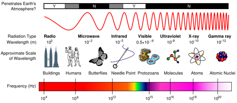
Almost every analytical procedure in this course comes down to the interaction of electromagnetic radiation with chemical species to produce a unit of measure. Different regions of the spectrum carry different amounts of energy and therefore probe different things — molecular rotations and vibrations in the infrared, valence electrons in the UV–visible, nuclear spin states in NMR, core electrons and nuclei at X-ray and γ-ray energies. Choosing a technique is choosing which energy levels you interrogate.
Two broad modes of measurement:
Direct measurement — light in, signal out, with little or no sample preparation: near-infrared (NIR), infrared (IR), UV, visible, Raman. The result often comes from a model over a whole spectrum rather than a single wavelength — which is exactly what Q2(R2)’s multivariate section addresses.
Separation first — resolve the mixture, then measure what comes off: thin-layer chromatography (TLC), HPLC/UHPLC, capillary electrophoresis (CE), gas chromatography, usually with a spectroscopic or mass-spectrometric detector at the end.
The validation characteristics are the same either way. What differs is where the variability enters the measurement system — and that is what shapes the validation design.
What are we trying to prove?
The fundamental question is: is the method fit for purpose? — and different purposes demand different demonstrations. An identity test has a different job from an assay; an assay has a different job from an impurity method; an impurity method at a 0.05 % reporting threshold has a different challenge from a dissolution test.
There is no universal validation package that every method must satisfy in the same way.
Q2(R2) sets the expected characteristics but explicitly permits scientifically justified alternative approaches, and it ties the validation strategy to the intended purpose and to what is already known about the procedure. It applies particularly to procedures used for release and stability testing; its scientific principles apply phase-appropriately during development and to other procedures in a control strategy.
Types of analytical procedure to be validated
Q2 organizes everything around four procedure types, because the validation you owe depends on the job the procedure does:
Type
What it does
Identification test
Confirms the identity of an analyte in a sample — normally by comparing a property of the sample (spectrum, chromatographic behaviour, chemical reactivity) against a reference standard.
Quantitative test for impurities
Measures the amount of an impurity present, to reflect the purity of the sample.
Limit test for impurities
Decides only whether an impurity is above or below a threshold — no exact value. It needs a different set of characteristics from the quantitative test.
Assay — quantitative test of the active moiety
Measures the content or potency of the major component: the drug substance, or the active (or another selected component) in the drug product. The same characteristics extend to assays behind other procedures, such as dissolution.
Identification tests ensure the identity of an analyte — the sample property is matched to that of a reference standard.
Impurity testing — quantitative or limit — must accurately reflect the purity characteristics of the sample. A quantitative test and a limit test require different validation characteristics: the quantitative test has to be accurate and precise at low levels; the limit test only has to detect reliably at the limit.
Assay procedures measure the analyte present in a sample. For the drug substance the assay quantifies the major component; for the drug product the same characteristics apply when assaying the active or another selected component, and also to assays associated with procedures such as dissolution.
The performance characteristics — the analytical figures of merit
These are the vocabulary of Q2 — the analytical figures of merit. Defining each one for a given method describes the design space in which the method can effectively operate and measure the quality of the process. Each is a different way of interrogating the measurement system — not a checklist to complete mechanically. Know these cold; they are the concept most likely to be tested.
Characteristic
The question it asks
Specificity / selectivity
Are we measuring what we think we’re measuring, in the presence of everything else?
Response
How does the analytical signal behave as concentration changes? (subsumes the former linearity)
Range
Over what concentration interval does the method perform suitably?
Accuracy
How close is the result to the true or accepted reference value?
Precision
How much do repeated measurements vary — within a run, across days/analysts, across labs?
Detection limit (DL)
At what level can we reliably tell an analyte is present?
Quantitation limit (QL)
At what level can we reliably measure how much is present?
Robustness
How sensitive is the method to small, deliberate changes in operating conditions?
Q2(R2) reorganizes some of this. Linearity is folded into response; the working range is discussed in terms of a reportable range tied to the intended use rather than a generic instrument property; selectivity/specificity are treated together; and the guideline adds explicit coverage of multivariate procedures and of stability of solutions and samples as part of the package.
The classic Q2 list — the one to memorize — is:
Accuracy
Precision — repeatability and intermediate precision (and, between laboratories, reproducibility)
Specificity
Detection limit
Quantitation limit
Linearity
Range
The figures of merit — formal definitions
These are the definitions to be able to state precisely:
Term
Definition
Accuracy
The closeness of agreement between the value which is accepted either as a conventional true value or an accepted reference value, and the value found.
Precision
The closeness of agreement (degree of scatter) between a series of measurements obtained from multiple sampling of the same homogeneous sample under the prescribed conditions. Considered at three levels: repeatability, intermediate precision, reproducibility.
Repeatability
Precision under the same operating conditions over a short interval of time. Also termed intra-assay precision.
Intermediate precision
Within-laboratory variation: different days, different analysts, different equipment.
Reproducibility
Precision between laboratories (collaborative studies, usually for standardization of methodology).
Specificity
The ability to assess unequivocally the analyte in the presence of components which may be expected to be present — typically impurities, degradants, matrix. A lack of specificity in one procedure may be compensated by other supporting procedure(s).
Detection limit (LOD)
The lowest concentration of analyte that can be determined to be statistically different from a blank — detected, but not necessarily quantitated as an exact value.
Quantitation limit (LOQ)
The lowest level above which quantitative results may be obtained with a specified degree of confidence (acceptable accuracy and precision).
Linearity
The ability of the procedure (within a given range) to obtain test results which are directly proportional to the concentration (amount) of analyte in the sample.
Range
The interval between the upper and lower concentration of analyte (inclusive) for which the procedure has been demonstrated to have a suitable level of precision, accuracy and linearity.
The three implications of specificity, by test type:
Identification — establish that the procedure identifies the analyte and does not respond to related structures.
Purity tests — establish that the procedures allow an accurate statement of the content of impurities (related substances, heavy metals, residual solvents, etc.).
Assay (content / potency) — establish that the procedure gives a result that allows an accurate statement of the content or potency of the analyte in the sample.
Which characteristics for which test type
The historical Q2 table — still the working mental model — maps characteristics to purpose. + = normally required, – = normally not.
Characteristic
Identification
Impurities — quantitative
Impurities — limit
Assay / content / dissolution
Specificity / selectivity
+
+
+
+
Accuracy
–
+
–
+
Precision — repeatability
–
+
–
+
Precision — intermediate
–
+
–
+
Detection limit
–
–
+
–
Quantitation limit
–
+
–
–
Response / linearity
–
+
–
+
Range
–
+
–
+
Read it as logic, not as a grid to memorize: an identity test only has to be specific; a limit test for an impurity has to detect reliably at the limit but need not quantify; a quantitative impurity method has to do nearly everything an assay does, plus work down at the reporting threshold.
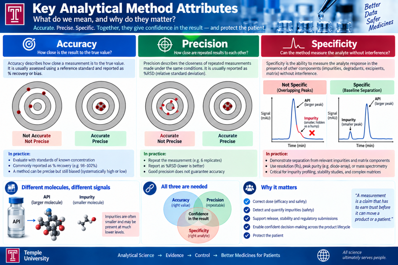
Specificity — “are we measuring the right thing?”
An API peak can look clean, integrate cleanly, and report 99.2 % while a degradation product co-elutes underneath it. The instrument still produces a number; the number may be wrong.
Specificity/selectivity is the evidence that the procedure distinguishes the analyte from everything relevant that could interfere:
impurities and degradation products
excipients and process-related materials
matrix components
other analytes measured by the same method
This is the hinge back to Q1: Q1 tells us the product may degrade; specificity is what lets the analytical procedure see that degradation correctly. Peak purity by diode-array and LC–MS, resolution from forced-degradation products, and mass balance are the usual evidence.
Accuracy — “are we getting the right answer?”
Accuracy is closeness of the measured result to an accepted reference or true value. Depending on the procedure it is shown with:
certified reference materials
spiking / recovery studies (add a known amount of analyte or impurity to the matrix, measure what comes back)
comparison against an orthogonal procedure
for an assay, from precision + specificity + response taken together
Spike 0.50 % of an impurity into the product matrix and recover 0.50 % consistently, and you have evidence the method is accurate in that region. But accuracy alone is not enough — a method can be accurate on average while being wildly variable.
Precision — “would I get the same answer again?”
Precision is the variability of repeated measurements, assessed at nested levels:
Level
What varies
Also called
Repeatability
Same analyst, same instrument, short interval
Intra-assay precision
Intermediate precision
Different days, analysts, instruments — one lab
Within-laboratory reproducibility
Reproducibility
Different laboratories
Inter-laboratory (method transfer / pharmacopoeial studies)
The target picture makes the accuracy/precision distinction concrete — they are independent axes:
Not accurate, not precise — shots scattered all over: neither the right answer nor a consistent one.
Accurate, not precise — shots average on the bullseye but scatter widely: right on average, but any single result could be well off.
Not accurate, precise — a tight cluster, but off-centre: consistently the wrong answer — the dangerous case, because the low scatter looks reassuring.
Accurate and precise — a tight cluster on the bullseye. This is the goal.
Accuracy is closeness to the right answer; precision is consistency. You need both, and Q2 asks for them separately.
Range — “where does this method actually work?”
A method is not equally reliable at every concentration. An impurity method intended for 0.05 % → 1.0 % may behave beautifully at 0.5 % and still not be demonstrated at 0.05 %. Validation has to cover the reportable range relevant to the intended use — for an assay typically 80–120 % of nominal, wider for content uniformity, down to the reporting threshold for impurities.
Q2(R2) makes reportable range an explicit concept: the interval over which the procedure has been shown to provide results of acceptable accuracy and precision for the decision it supports, not a generic property of the instrument.
Detection limit vs. quantitation limit
Students routinely conflate these:
Claim
Typical basis
Detection limit
“I can tell something is there.”
Signal-to-noise ≈ 3:1; or from the response SD and slope
Quantitation limit
“I can measure how much is there, with acceptable accuracy and precision.”
Signal-to-noise ≈ 10:1; confirmed by accuracy + precision at that level
Seeing a small peak at 0.01 % does not license reporting Impurity = 0.010 %. The ability to see something and the ability to measure it are different scientific claims, and the QL — not the DL — has to sit at or below the reporting threshold for a quantitative impurity method.
Robustness — “what happens when reality isn’t perfect?”
Real laboratories are not perfectly controlled: mobile-phase preparation varies, column temperature drifts, pH moves, flow rate is never mathematically exact, different analysts prepare samples, different instrument units behave differently. Robustness asks whether the method stays fit for purpose under small, deliberate, reasonable variations in those factors.
This is the connection to Q14 and the enhanced approach:
Robustness is not something you discover accidentally during validation. It is something you should establish during development — ideally by design of experiments — so the method arrives at validation with a known operable region.
A fragile method can pass validation under ideal conditions and then be a nightmare in routine QC.
Precision is not the same as reproducibility
Worth a few minutes with graduate students. Lab A runs the method and gets 99.1, 99.2, 99.1, 99.2 %. Lab B gets 98.9, 99.4, 99.0, 99.3 %. Now transfer the method to five manufacturing sites: if every site produces a slightly different answer, you have a method deployment problem, not necessarily a product problem.
The goal is not “the method worked in the development laboratory.” The goal is “the measurement system stays fit for purpose wherever it is legitimately used” — which is why method transfer and lifecycle management (see Quality Control) matter as much as the original validation.
Stability-indicating methods
This is the deepest link to the Q1 lecture. A stability-indicating procedure must be able to detect and quantify the relevant changes in the product over time. The workflow:
stress the product → generate degradation products → develop the analytical separation → demonstrate specificity against those degradants → evaluate assay + degradants → check mass balance → validate the procedure → deploy it in the stability program
So Q1 and Q2 interlock:
Q1 — the product changes.
Q2 — the measurement system can detect and quantify the change.
Q2(R2) specifically addresses demonstration of stability-indicating properties as part of specificity/selectivity.
Validation samples are experiments
A teaching point: don’t say “now we do validation.” Say “now we design experiments that let us make defensible claims about the performance of the measurement system.” For example —
Claim
The method is accurate across 80–120 % of nominal concentration.
Experiment
Prepare samples at known concentrations spanning that range.
Evidence
Compare measured results against the accepted values.
Conclusion
Decide whether the observed performance supports the claim.
That is the hypothesis → experiment → data → interpretation → conclusion → revision loop from Section 1, applied to the measurement instead of the molecule.
Statistics are part of analytical science
Q2 is where students should stop seeing statistics as decoration added to a report at the end. Statistics answer: how variable is the method? is an observed difference meaningful? is the response behaving as expected? what range is supported? are results consistent across analysts, days, instruments? how much confidence belongs on the estimate?
Two cautions:
A statistically significant result is not automatically scientifically important.
A non-significant result does not prove two things are identical.
The analyst interprets the statistics against the intended analytical purpose — that judgment is the A in STEAM.
Multivariate analytical procedures
Modern analytical science increasingly goes beyond one signal and one concentration — NIR, Raman, chemometrics, multivariate calibration, process analytical technology. Here the result comes from a model, not a single peak, and Q2(R2) adds explicit considerations for these procedures.
The question for students: when the result comes from a model, what exactly are we validating? Not just the instrument, not just the spectrum — the measurement system and the model together, including how the model was trained, how its inputs are controlled, and how it will be maintained as the process and the samples drift.
Platform methods change the equation
If a company already has a well-understood analytical platform and develops another molecule using essentially the same approach, it does not have to start validation from zero. Q2(R2) recognizes that a platform analytical procedure applied to a new purpose can be validated with an abbreviated package when scientifically justified.
The QbD principle underneath: knowledge has value. Accumulated, reliable knowledge about a measurement platform should not be discarded every time a new product enters development.
Validation through the lifecycle
The most important modernization in how Q2 is taught:
A method can drift. Instruments change, column suppliers change, the formulation changes, the process changes, the impurity profile changes, the specification changes, technology improves. Therefore:
The validated state is not a frozen state.
Validation is evidence that the procedure is fit for purpose at a point in its lifecycle. The procedure then needs monitoring and maintenance — continued performance verification — for the rest of its useful life, and Q2(R2) places that explicitly inside the Q14 lifecycle.
The Q2 → Q14 → QC map
Put this on the board instead of “Q2 is the validation guideline”:
Lifecycle management (Q12) — what do we do when the world changes?
Q14 builds the scientific understanding; Q2 provides the framework for demonstrating performance; the lifecycle maintains the state of control.
The analytical procedure as a control
A QC result is a decision — pass → release, fail → investigate / reject / hold. The analytical procedure is not merely producing information; it participates in the control strategy. If the measurement is wrong, the decision can be wrong: a false pass releases a defective product; a false fail rejects good product. Behind that decision is a patient.
Analytical validation is ultimately about protecting the quality decision.
The hierarchy of confidence
A useful visual — each layer depends on the ones below it:
Question
Characteristic
Can I see it?
Detection limit
Can I measure it?
Quantitation limit
Am I measuring the right thing?
Specificity / selectivity
Am I getting the right answer?
Accuracy
Would I get the same answer again?
Precision
Does it work where I need it to?
Reportable range
Does it survive reasonable variation?
Robustness
Can I defend the result?
Validated analytical procedure
What Q2 does not mean
Students often take away the wrong impression. Q2 does not mean:
“Do these nine tests and you’re validated.”
“Every method needs exactly the same experiments.”
“A passing validation report proves the method will work forever.”
“The instrument is qualified, therefore the analytical result is valid.”
Instead: validation is a scientifically justified body of evidence that the analytical procedure is fit for its intended purpose. That distinction is the heart of Q2(R2).
Where the analyst sits
Every number in a development or QC report ultimately rests on a measurement. The analyst is not asking “what number did the instrument produce?” but “what does this number mean, and what evidence lets me trust it?” — which draws on chemistry, instrumentation, statistics, experimental design, risk assessment, judgment, documentation, and scientific integrity at once. That is STEAM in action.
If the Q1 lesson is a shelf life is a hypothesis that must survive testing, the Q2 lesson is a measurement is a claim that must earn our trust — and together they run the sequence the course follows: science → Q1 stability → Q2 validation → Q3 impurities → Q6 specifications → Q8–Q14 quality by design. The thread is not memorizing guidelines; it is answering how do we know? and then how do we know that we know?
For discussion
An assay reports 99.2 % and the chromatogram looks clean. What specific evidence would convince you a degradation product is not hiding under the main peak?
An impurity method has a quantitation limit of 0.08 % and a reporting threshold of 0.05 %. Is the method fit for purpose? What are the options?
You validated a method in the development lab; two manufacturing sites now get results that differ by 1.5 %. Is this a product problem, a method problem, or a transfer problem — and what data tells you which?
Your company has a platform HPLC assay used on six prior molecules. A regulator asks why the validation package for molecule seven is abbreviated. What is the scientific justification, and where are its limits?
A NIR method predicts assay from a chemometric model. List everything that is “the measurement system” here, and say what you would monitor over the method’s life.
Forced degradation (from the Q1 workflow) produces a degradant at 80 °C that never appears at 25 °C. Does your method need to resolve it? Does it belong in the specificity package?
A validation result is statistically significant but the effect is 0.2 % of nominal. A different result is non-significant with a 3 % spread. Which one worries you, and why?
Source note. ICH Q2(R2) Validation of Analytical Procedures reached Step 4 on 1 November 2023 and is the current guideline; a minor error-correction version was issued in 2025. Its stated objective is to demonstrate that an analytical procedure is fit for its intended purpose, and it is explicitly harmonized with Q14 and the analytical-procedure lifecycle. Primary texts: the ICH Q2(R2) guideline (2023) and the 2025 error-correction version. (Instructor: confirm the current characteristic-by-test-type table against the R2 text before lecture — the guideline reframes linearity/range as response and reportable range.)
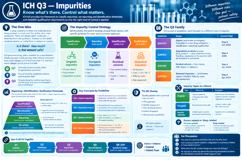
1.3.3 - ICH Q3 — Impurities
A deep dive into the Q3 family: what counts as an impurity and how impurities are classified (organic — process- and drug-related, inorganic, residual solvents), the reporting / identification / qualification threshold ladder and why it scales with daily dose, Q3A for the drug substance and Q3B for degradation products in the drug product, what qualification and identification actually demand of the analyst, Q3C residual solvents (the four classes, PDE, Option 1 vs Option 2, the R9 volatility update), Q3D elemental impurities (24 elements, the class 1/2A/2B/3 scheme, PDEs by route, the 30 % control threshold, the risk assessment that replaced USP <231>), the M7 mutagenic-impurity overlay (TTC, (Q)SAR, the five structural classes, the cohort of concern, nitrosamines and M7(R3)), and how the whole set feeds the specification (Q6) and the analytical method (Q2).
The one idea
A drug substance is never one molecule and a drug product is never just the active plus inert excipients. Alongside the thing you are selling there is always a population of other molecules — leftovers from the synthesis, things the molecule turned into on the shelf, solvent that never fully dried off, metal from a catalyst or a reactor wall. Every one of them is a question:
Is it there? How much? Is that amount safe?
Q3 is the framework that answers the third question by turning toxicology into a number on a specification. It says, for a given impurity at a given patient exposure, how much you may ship without further comment, how much obliges you to find out what it is, and how much obliges you to prove it is safe.
This pairs with the two sections before it:
Q1 asks: does the product remain within its specification over time?
Q2 asks: can we trust the analytical evidence used to answer that?
Q3 asks: of everything the method sees that is not the drug, how much is acceptable — and on what basis?
What counts as an impurity
An impurity is any component of the drug substance or drug product that is not the drug substance (or, in the product, an excipient). Q3 sorts them three ways:
Class
What it is
Where it comes from
Organic impurities
Carbon-containing molecules other than the API
Starting materials, by-products, intermediates, reagents, ligands, catalysts, and degradation products
Reaction and crystallisation solvents that do not fully evaporate (→ Q3C)
Two cross-cutting distinctions matter more than the list:
Process-related vs. drug-related. A process impurity rides in from the synthesis and is (in principle) removed by better process control and purification — it is a Q11 problem, fixed upstream. A degradation product forms from the drug itself and grows over shelf life — it is a Q1 problem, and no amount of upstream purification removes it.
Specified vs. unspecified. A specified impurity has its own line and its own acceptance criterion on the specification (named, or identified by relative retention). Everything else is caught by two catch-all limits — “any unspecified impurity ≤ identification threshold” and “total impurities ≤ …”. This is the machinery Q6 assembles into the release contract.
The Q3 family
Q3 is not one document — it is a set, split by the kind of impurity:
Guideline
Scope
Current step
Q3A(R2)
Organic (and a note on inorganic) impurities in a new drug substance — classification, reporting, the threshold tables, qualification
Step 4, Oct 2006
Q3B(R2)
Degradation products in a new drug product — only what forms from the drug substance or from its reaction with an excipient or the container
Step 4, 2006
Q3C(R9)
Residual solvents — the four solvent classes, permitted daily exposure (PDE), Option 1 / Option 2 limits
Step 4, Jan 2024
Q3D(R2)
Elemental impurities — 24 elements, class 1 / 2A / 2B / 3, PDEs by route of administration, the risk-assessment process
Step 4, Apr 2022
M7(R2)
Mutagenic (DNA-reactive) impurities — a Multidisciplinary guideline, not a “Q”, but the class should know it sits with Q3
Step 4, Apr 2023
The mental model: Q3A/Q3B set the general rules for “ordinary” impurities; Q3C, Q3D and M7 carve out three categories that need their own toxicology because a percentage-of-the-API limit is the wrong tool for them.
The challenge: a moving target
The same difficulty that shadows Q1 and Q2 applies here. The impurity profile is a function of the process, and the process changes throughout development — a new route, a new supplier of a starting material, a scale-up, a site change, a different final crystallisation. Each change can add an impurity, remove one, or shift a ratio. An impurity that was below the reporting threshold in the tox batches can appear at 0.2 % in the first commercial-scale lot.
When everything around the molecule is changing, standardise how you track what is not the molecule.
The defence is the same discipline Q1 and Q2 demand: a fixed, validated, specific method that resolves the known impurities, a fixed reporting convention, and a documented impurity fate map so that when a new peak appears you can say whether it is new chemistry or a known impurity that moved.
The core concept: three thresholds
This is the idea to fix for graduate students. For any impurity, its measured level falls into one of four bands, and the band — not a single universal limit — dictates what you owe:
Band
Level
What is required
Below the reporting threshold
trace
Nothing — it need not even appear in the registration application
At or above reporting, below identification
small
Report the actual result (a number, not “< X”) in the batch analyses
At or above identification, below qualification
moderate
Identify the impurity — establish its structure
At or above qualification
large
Qualify it — provide data establishing biological safety at that level
Two features make this elegant rather than arbitrary:
The thresholds scale with exposure. They are expressed as a percentage of the drug substance or as an absolute daily intake (µg or mg per day), whichever is lower. A 5 mg tablet and a 1 g tablet do not get the same percentage limit, because the patient’s actual dose of the impurity is what matters.
The ladder is cumulative. Anything you must qualify, you must first have identified and reported. Each rung is a stricter scientific claim: I saw it → I know what it is → I know it is safe.
Q3A — impurities in the new drug substance
Q3A(R2) applies to the drug substance made by chemical synthesis (not biologics — that is Q6B). It asks the applicant to:
Summarise the actual and potential impurities most likely to arise from the synthesis, purification, and storage, with a rationale for each based on the chemistry;
List the impurities found in development and toxicology batches, with the analytical procedures used;
Classify each as an identified/unidentified organic impurity, a residual solvent, or an inorganic impurity;
Set acceptance criteria for individual specified impurities, any unspecified impurity, and total impurities.
The threshold table (drug substance):
Maximum daily dose
Reporting threshold
Identification threshold
Qualification threshold
≤ 2 g/day
0.05 %
0.10 % or 1.0 mg/day intake (whichever is lower)
0.15 % or 1.0 mg/day intake (whichever is lower)
> 2 g/day
0.03 %
0.05 %
0.05 %
Read the “>2 g/day” row as the safety net: at very high doses even a small percentage is a large absolute intake, so the thresholds tighten.
Q3B — degradation products in the new drug product
Q3B(R2) is deliberately narrower than Q3A. In the finished product it covers only:
degradation products of the drug substance formed during manufacture or storage of the product, and
reaction products of the drug substance with an excipient or with the container closure system.
It explicitly does not cover: impurities carried in from the drug substance process, impurities in the excipients themselves, extractables/leachables (a separate discipline), or polymorphic and enantiomeric changes. The logic: the product-stability method should be watching for new chemistry that happens after the drug substance is released — which is exactly the stability-indicating capability that Q1 forced degradation and Q2 specificity exist to demonstrate.
The threshold tables (drug product) are more granular than Q3A because product doses span a wider range. “TDI” is the total daily intake of the degradation product, and “whichever is lower” always applies.
Reporting threshold:
Maximum daily dose
Threshold
≤ 1 g
0.1 %
> 1 g
0.05 %
Identification threshold:
Maximum daily dose
Threshold
< 1 mg
1.0 % or 5 µg TDI
1 mg – 10 mg
0.5 % or 20 µg TDI
> 10 mg – 2 g
0.2 % or 2 mg TDI
> 2 g
0.10 %
Qualification threshold:
Maximum daily dose
Threshold
< 10 mg
1.0 % or 50 µg TDI
10 mg – 100 mg
0.5 % or 200 µg TDI
> 100 mg – 2 g
0.2 % or 3 mg TDI
> 2 g
0.15 %
Qualification — turning a number into a safety judgment
Qualification is the process of acquiring and evaluating data that establishes the biological safety of an individual impurity or a given impurity profile at the level(s) specified. It is not automatically a new toxicology study. The Q3A/Q3B decision tree offers, roughly in order of preference:
Is the level already covered? If the impurity is also a significant metabolite of the drug, or is present at a comparable level in a batch already tested in humans or animals, it is considered qualified.
Is it below the qualification threshold? Then no action is needed unless it carries a structural alert for unusual toxicity or genotoxicity (→ M7).
If above the threshold and not otherwise qualified: reduce it (better process or formulation), or generate data — typically a genotoxicity screen (bacterial mutagenicity + one chromosomal-damage assay) and a general toxicity study (usually ≥ 14 days, in a relevant species) at a dose that gives the required exposure margin.
The teaching point: qualification is a risk-based off-ramp, not a mandatory battery. Most impurities are qualified by argument and existing data; only the genuinely novel, genuinely abundant ones drive new studies.
Identification — what “identify” actually demands
To “identify” an impurity is to establish its structure — not merely to give it a relative retention time and a code. This is step 7 of the degradant-profiling workflow from the Q1 lecture, and it uses the same tools:
Tool
What it gives
LC–MS / LC–MSn
Molecular formula from accurate mass; fragmentation map; often enough to propose a structure for a degradant related to a known parent
LC–NMR / preparative isolation + NMR
Connectivity and stereochemistry — needed when the mass is unchanged (isomerisation, rearrangement) or ambiguous
Preparative chromatography / synthesis of the authentic standard
A reference material to confirm identity by co-elution and to use for accurate quantitation
Orthogonal separation
Confirms one peak is one compound (peak purity), and that co-eluting impurities are not being missed
An unidentified impurity above the identification threshold is a finding the application has to explain: what was tried, why the structure could not be assigned, and why the safety argument still holds.
Q3C — residual solvents
Solvents are treated separately because their toxicity is known and dose-based, not a function of “percent of API”. Q3C(R9) sorts solvents into four classes:
Class
Meaning
Basis
Examples (limit)
Class 1
Avoid
Known/suspected human carcinogens; environmental hazards
Isopropyl ether, methylisopropyl ketone, petroleum ether — justify case by case
PDE (permitted daily exposure) is the anchor. It is derived from a no-effect level in the most relevant animal study, scaled to a 50 kg adult and divided by a stack of five safety factors (interspecies extrapolation, individual variability, short-study correction, severe-toxicity correction, and a NOEL-vs-LOEL adjustment):
PDE = (NOEL × 50 kg) / (F₁ × F₂ × F₃ × F₄ × F₅)
For Class 2 solvents there are two ways to set a limit:
Option 1 — a fixed concentration limit (ppm), computed assuming a maximum product intake of 10 g/day. Simple; conservative for low-dose products.
Option 2 — back-calculate an allowed concentration from the actual maximum daily dose of the product, so the daily amount of solvent meets the PDE. More generous when the real dose is well under 10 g.
R9 (minor revision, January 2024) added consideration of solvent volatility when choosing and validating the analytical method (headspace GC behaviour differs sharply between, say, methanol and DMSO), and refreshed the Annex decision trees.
Q3D — elemental impurities
Q3D(R2) replaced the century-old USP <231> heavy-metals test — a non-specific colorimetric sulfide-precipitation assay with poor and element-dependent recovery — with a risk-based, element-specific framework, implemented analytically by USP <232> (limits) and <233> (ICP-OES / ICP-MS procedures).
24 elements, four classes:
Class
Elements
Toxicity / occurrence
Assessment
1
As, Cd, Hg, Pb
Highly toxic; enter via mined/natural excipients and water
Required for all routes
2A
Co, Ni, V
Higher probability of occurrence
Required for all routes
2B
Ag, Au, Ir, Os, Pd, Pt, Rh, Ru, Se, Tl
Low probability unless intentionally added (catalysts)
Only if added
3
Ba, Cr, Cu, Li, Mo, Sb, Sn
Low oral toxicity (oral PDE > 500 µg/day)
Parenteral & inhalation routes
PDEs are set per route of administration — oral, parenteral, inhalation, and (added in R2) cutaneous and transcutaneous — because absorption differs by orders of magnitude. The control threshold is 30 % of the PDE: if an element is consistently below that across representative batches, no additional controls are needed.
The heart of Q3D is the risk assessment, not a test:
Identify known and potential sources — drug substance, each excipient, water, reagents, manufacturing equipment (reactor alloys, catalysts), container closure system.
Evaluate the likely contribution of each source against the PDE, using data, prior knowledge, and worst-case additivity.
Summarise and document the conclusion and any controls; test routinely only where the assessment cannot rule out a problem.
R2 (2022) revised the PDEs for gold, silver and nickel and added the cutaneous/transcutaneous routes.
Options for turning a PDE into a per-component concentration limit mirror Q3C: Option 1 (a common limit assuming 10 g/day intake), Option 2a (common limit at the actual daily dose), Option 2b (component-specific limits summing to the PDE), Option 3 (measure the finished product).
M7 — the mutagenic-impurity overlay
Some impurities are dangerous at levels far below any Q3A/Q3B threshold because they are DNA-reactive — a single molecule can cause a mutation. A “0.10 %” identification threshold is meaningless for a compound whose safe intake is measured in micrograms per day. M7(R2) handles these.
Acceptable intake: the threshold of toxicological concern (TTC) of 1.5 µg/day, corresponding to a theoretical excess lifetime cancer risk of 1 in 100 000.
Hazard assessment: database and literature search, then two complementary (Q)SAR methodologies — one expert rule-based, one statistical. Concordance (or an expert overruling) drives the call.
Five structural classes:
Class
Definition
Control
1
Known mutagenic carcinogen
Compound-specific limit
2
Known mutagen (bacterial), carcinogenicity unknown
≤ TTC
3
Structural alert, unrelated to the drug substance, no data
≤ TTC, or run a bacterial mutagenicity assay → if negative, treat as Class 5
4
Structural alert shared with the (non-mutagenic) drug substance
Treat as a non-mutagenic impurity — Q3A/Q3B
5
No structural alert, or data show no mutagenicity
Treat as a non-mutagenic impurity — Q3A/Q3B
Cohort of concern — N-nitroso compounds, aflatoxin-like compounds, alkyl-azoxy compounds — are so potent that the generic TTC does not protect; they need compound-specific limits derived from their own carcinogenicity data.
M7(R3), in progress — folds in an N-nitrosamine addendum built on the Carcinogenic Potency Categorisation Approach (CPCA), which scores a nitrosamine’s structural features to place it in a potency category and assign an acceptable intake. This is the ICH response to the 2018-onward nitrosamine recalls (valsartan/NDMA, ranitidine/NDMA).
How the pieces fit — the impurity control strategy
Q3 is not read in isolation; it is one layer of a control strategy that runs the length of the course:
Q11 — choose starting materials and design the route so that process impurities are formed late enough, or purged efficiently enough, to be controlled
↓
Q3A / Q3C / Q3D — characterise and limit the process impurities, residual solvents, and elemental impurities that remain in the drug substance
↓
Q1 — forced degradation and stability studies reveal which impurities grow over shelf life
↓
Q3B — limit the degradation products in the finished product; M7 overlays a stricter limit on any impurity or degradant that is DNA-reactive
↓
Q6 — assemble the acceptance criteria into the release specification: specified impurities, unspecified-impurity limit, total impurities
↓
Q2 — validate the method that has to see every one of these at its limit, batch after batch
What Q3 demands of the analytical method
Every Q3 number is only real if a method can measure it. The chain of consequences for the analyst:
Sensitivity. The quantitation limit must sit at or below the reporting threshold — you cannot report “0.06 %” from a method whose QL is 0.1 %. This is the direct link to the Q2 detection/quantitation-limit discussion.
Specificity. Each specified impurity must be resolved from the API and from every other specified impurity; peak purity has to be demonstrated for the main peak and for any impurity used to set a limit.
Relative response factor (RRF). An impurity quantified against the API peak is only accurate if its detector response per unit mass is known. Either measure the RRF and apply a correction, or demonstrate the response is equivalent (within, say, 0.8–1.2) and quantify directly. An unknown RRF is an unstated systematic error in every impurity result.
Mass balance. The drop in assay should be accounted for by the rise in degradation products. A gap means an impurity the method is not seeing — a specificity failure hiding as a clean chromatogram.
Where the analyst sits
An impurity result is a small number attached to a large decision. Deciding whether “0.12 %” of a late-eluting peak is a known process impurity or a new degradant; whether the RRF assumption still holds after a formulation change; whether an unidentified 0.11 % peak needs a structure or a better argument; whether a structural alert turns an ordinary impurity into an M7 problem — these are analytical judgments, drawing on synthetic chemistry, spectroscopy, toxicology literacy, statistics, and documentation at once. That is the A in STEAM: the science produces the peak; the analyst decides what it means and what the patient’s exposure to it should be allowed to be.
If the Q1 lesson is a shelf life is a hypothesis that must survive testing, and the Q2 lesson is a measurement is a claim that must earn our trust, the Q3 lesson is: an impurity limit is a safety argument in the form of a number — and the analyst is the person who has to be able to defend it.
For discussion
A tablet contains 5 mg of API; a capsule of the same drug contains 800 mg. An impurity is present at 0.12 % in both. What does each product owe under Q3B, and why are the answers different?
Your drug-substance process changes suppliers for a key starting material and a new impurity appears at 0.18 %. Walk through the reporting / identification / qualification decisions. What data would qualify it fastest?
An impurity is a known human metabolite of the drug, present at 0.4 % in the drug substance (qualification threshold 0.15 %). Is it qualified? What is your argument?
A degradation product co-elutes with the API and is only revealed by an orthogonal method. Which Q3B obligations were you failing to meet while the method was non-specific, and what has to be re-done?
Your method quantifies all impurities against the API peak with an assumed RRF of 1.0. One impurity turns out to have an RRF of 0.4. Which reported results were wrong, and in which direction?
A structural-alert check flags one specified impurity as class 3 under M7. It is currently controlled at 0.10 %. What changes?
Residual DMF is at 700 ppm; the Class 2 Option 1 limit is 880 ppm but your product’s maximum daily dose is only 200 mg. Is Option 2 worth the paperwork here?
A regulator asks why your Q3D risk assessment does not include routine testing for palladium, even though a Pd catalyst is used two steps before the final intermediate. What is your answer, and what evidence backs it?
The Q4 family and the compendial baseline: what a pharmacopoeia is and how a monograph differs from a general chapter, the three ICH-region pharmacopoeias (USP–NF, Ph. Eur., JP) and the Pharmacopoeial Discussion Group that harmonises their shared texts, why full harmonisation (Q4A) stalled and the evaluate-and-recommend mechanism (Q4B) that replaced it, what ‘interchangeable’ actually means and the region-specific text that remains, the fourteen Q4B annexes and the general chapters they cover, and what compendial status demands of the analyst — verification under USP <1226>, the rules for a validated alternative method, and when the compendial method is mandatory.
(The graphic is a lecture aid, not a citation — its “Q4C / Q4D / Q4E” rows and some panel labels don’t match the current ICH text; the Q4 family is Q4B plus its fourteen annexes, as described below.)
The one idea
Q1, Q2 and Q3 are about methods you develop and defend. Q4 is about the methods you didn’t — the shared, published tests that every pharmacopoeia already prescribes for sterility, dissolution, endotoxins, uniformity of dosage units, residue on ignition, and dozens more. These are the compendial baseline: a company does not re-invent a sterility test, it runs the one in the book.
The problem Q4 addresses is that there is more than one book.
The USP sterility test, the Ph. Eur. sterility test, and the JP sterility test all measure the same thing. If they are written differently, a manufacturer selling in all three regions may have to run the test three times — three protocols, three validations, three sets of records — for no gain in product quality.
Q4 is the framework for making one test count everywhere. Its lesson: harmonisation is a quality tool — it removes duplicated work that adds cost and risk without adding assurance.
What a pharmacopoeia is
A pharmacopoeia is a legally recognised compendium of standards for medicines: what a substance or product must be, and the tests that demonstrate it. In a filing, citing a pharmacopoeial standard means you are held to that text as published, including its future revisions.
Two kinds of text, and the distinction runs through the rest of this page:
Monograph
General chapter
Scope
One specific article — a named drug substance, excipient, or dosage form
A method or policy shared across many articles
Contains
Definition, identification, assay, impurity limits, specific tests — the specification for that article
How to perform a test (dissolution apparatus, endotoxin assay), or a general requirement
Example
Ibuprofen Tablets
<711> Dissolution, <85> Bacterial Endotoxins Test
In USP, the chapter number signals enforceability: chapters numbered below <1000> are requirements; <1000> and above are informational. Ph. Eur. and JP use their own numbering but draw the same line between mandatory methods and guidance.
Q4 is overwhelmingly about general chapters — the shared methods — because that is where harmonisation is both feasible and valuable. Monographs are article-by-article and largely left to the individual pharmacopoeias.
The three pharmacopoeias and the PDG
The ICH regions are served by three pharmacopoeias:
Region
Publisher
USP–NF
United States
United States Pharmacopeial Convention
Ph. Eur.
Europe (38 member states)
EDQM, Council of Europe
JP
Japan
MHLW / PMDA
Since 1989 these three have coordinated through the Pharmacopoeial Discussion Group (PDG) — a body separate from ICH whose job is to write harmonised versions of shared general chapters and excipient monographs. The PDG works a topic through a multi-stage process (identification → investigation → expert-committee draft → public consultation → consensus → regional adoption → ongoing maintenance), and a text is “PDG-harmonised” only when all three pharmacopoeias have adopted substantively the same wording. WHO participates as an observer. A PDG reform, published in 2021, opened a pilot to admit further pharmacopoeias; the Indian Pharmacopoeia Commission joined that pilot from 2022.
PDG harmonises the text. ICH’s role (Q4B) is to tell regulators the harmonised text can be relied on. Those are two different jobs done by two different bodies.
The Q4 family
Guideline
Scope
Status
Q4
Pharmacopoeias — the umbrella topic
Framework only
Q4A
Pharmacopoeial harmonisation — the original ambition of a single harmonised text set
Not pursued as an ICH guideline; the work sits with the PDG
Q4B
Evaluation and recommendation of pharmacopoeial texts for use in the ICH regions
Core guideline Step 4, November 2007
Q4B Annexes 1–14
One PDG-harmonised general chapter each, evaluated and recommended by the Q4B Expert Working Group
Step 4, 2009–2013
Q4A — why “one text” stalled
The tidy end-state would be a single harmonised pharmacopoeial text adopted verbatim by every region. In practice that runs into:
Legal standing. Each pharmacopoeia is embedded in its own region’s law. A pharmacopoeia cannot simply cede authorship of a legally binding standard to an external group.
Format and general-notices differences. Reagents, reference standards, rounding rules, and the “general notices” that govern how every monograph is read differ between compendia; a chapter that is word-identical can still behave differently inside its parent book.
Revision cycles. The three pharmacopoeias publish on different schedules, so even a jointly agreed text drifts out of alignment over time unless actively maintained.
So ICH did not produce a Q4A guideline. Instead it accepted that the PDG would keep harmonising texts as far as practical, and built Q4B to get regulatory value out of that work without requiring perfect textual identity.
Q4B — evaluate and recommend
Q4B set up an Expert Working Group with members from the three regulatory authorities and the three pharmacopoeias. Its process, per harmonised general chapter:
The PDG declares a general chapter harmonised (Stage 5/6 of its process).
The Q4B EWG evaluates that text: are the three pharmacopoeial versions technically equivalent for regulatory purposes? Where do real differences remain?
The EWG issues an annex with a formal outcome — typically that the texts are interchangeable, so a manufacturer may use any one of the three and it will be accepted by regulators in all three ICH regions.
The annex records region-specific conditions: passages that are not harmonised, additional local requirements, or parts of the chapter the recommendation does not cover.
“Interchangeable” is the payoff: run the Ph. Eur. dissolution chapter, cite it in a US or Japanese submission, and it is accepted — you do not re-run it to USP <711>. But interchangeable is not “identical.” Ph. Eur. marks non-harmonised passages with black diamonds (♦…♦); USP uses a similar convention. The Q4B annex is where you learn which parts of a chapter you can actually rely on across regions and which still carry a regional tail.
The Q4B annexes
Each annex is one general chapter. The fourteen:
Annex
General chapter
1
Residue on Ignition / Sulphated Ash
2
Test for Extractable Volume of Parenteral Preparations
3
Test for Particulate Contamination: Sub-visible Particles
4A
Microbiological Examination of Non-Sterile Products: Microbial Enumeration Tests
4B
Microbiological Examination of Non-Sterile Products: Tests for Specified Micro-organisms
4C
Microbiological Examination of Non-Sterile Products: Acceptance Criteria
5
Disintegration Test
6
Uniformity of Dosage Units
7
Dissolution Test
8
Sterility Test
9
Tablet Friability
10
Polyacrylamide Gel Electrophoresis
11
Capillary Electrophoresis
12
Analytical Sieving
13
Bulk Density and Tapped Density of Powders
14
Bacterial Endotoxins Test
The pattern is clear: these are workhorse release and characterisation tests — the ones almost every solid oral, parenteral, or biologic filing has to include. Harmonising them removes duplicated method work from nearly every dossier. Note what is absent: chromatographic assay methods, spectroscopy, and anything close to a specific molecule — those stay in monographs, where harmonisation is far harder and the ICH quality guidelines (Q2, Q3, Q6) do the heavy lifting instead.
The compendial-method obligations for the analyst
Q4 is where “a method in the book” meets “a method in your lab.” Three rules govern that hand-off.
1. Verification, not validation, for a compendial method. A pharmacopoeial method is already validated by the pharmacopoeia. When you adopt one, you do not re-run a full Q2 package — you verify it works in your hands, with your product matrix, on your instruments. USP <1226> Verification of Compendial Procedures frames this: assess the subset of Q2 characteristics that could plausibly fail on transfer — usually specificity against your impurities and excipients, and precision — and document it. Verification is lighter than validation precisely because someone else already did the validation.
2. A validated alternative is allowed — but the compendial method wins ties. You may use an alternative (often faster, or better suited to your matrix) provided you demonstrate equivalence to the compendial method. The catch: in a dispute, the pharmacopoeial method is the referee. If your rapid microbiological method and the <71> sterility test disagree, the compendial result stands. So an alternative method needs a validation package and an equivalence argument, and you still have to be able to run the compendial method.
3. Sometimes the compendial method is mandatory. Where a monograph or a regulation names a specific test as the standard — many endotoxin, sterility, and elemental-impurity requirements — that method is not optional and an alternative needs regulatory agreement, not just internal equivalence data. This is how Q3 reaches the bench: Q3C and Q3D set the limits, and USP <467> (residual solvents) and <232>/<233> (elemental impurities) are the compendial procedures that enforce them.
Harmonisation status — a moving target
The same caution that shadows Q1 and Q3 applies here: the compendial landscape moves.
The PDG reform (2021) restructured the harmonisation process and opened membership; the outcome of the expansion pilot is still settling.
ICH has signalled that the Q4B mechanism will not be extended to new general chapters — the reformed PDG process, with regulators engaged earlier, is expected to carry harmonisation forward, and the fourteen existing annexes remain in force.
Individual chapters are revised on their own cycles; a chapter that was harmonised can partly de-harmonise when one pharmacopoeia updates ahead of the others.
The practical consequence for a filing written today: check the current Q4B annex and the current version of each cited general chapter in all target regions, rather than assuming “harmonised” is permanent.
(Status as of early 2026 — confirm the PDG reform outcome and the Q4B forward plan against current ICH/PDG communications before lecture.)
How it fits the control strategy
Q4 is the layer that supplies the shared methods the rest of the framework assumes:
PDG — harmonise the general chapters (sterility, dissolution, endotoxins, uniformity …)
↓
Q4B — recommend the harmonised text as interchangeable across the ICH regions, with the regional caveats documented
↓
Q6 — the specification cites those chapters as the tests behind its acceptance criteria
↓
Q2 / USP <1226> — verify each adopted compendial method performs in your lab with your product
↓
Q7 / QC — run it, batch after batch, as part of the release decision
Where the analyst sits
Compendial methods can look like the boring part of the job — you follow the book. But the judgment calls are real: does this harmonised dissolution chapter’s non-harmonised apparatus footnote matter for my product in this region? Is my faster endotoxin method genuinely equivalent, or only equivalent on the batches I happened to test? Did the last Ph. Eur. supplement change a chapter I cite, and does my US filing still line up? The pharmacopoeia gives you the method; deciding whether it fits, whether an alternative is defensible, and whether your version still matches the current text across three regions is analytical work.
If the Q1 lesson is a shelf life is a hypothesis that must survive testing, and the Q2 lesson is a measurement is a claim that must earn our trust, the Q4 lesson is: a standard is only useful if everyone reads it the same way — and harmonisation is the unglamorous work of making that true.
For discussion
A harmonised general chapter is “interchangeable” under a Q4B annex, but the annex lists a region-specific acceptance criterion for one ICH region. You run the test once. Have you met the requirement everywhere? What do you check?
Your site wants to replace the compendial <71> sterility test with a rapid microbiological method. What does Q4 / compendial practice require before you can, and what must you still be able to do afterwards?
You adopt the PDG-harmonised Uniformity of Dosage Units chapter. Which Q2 characteristics would you include in the USP <1226> verification, and which would you skip — and why?
Why did ICH build Q4B (evaluate and recommend) instead of pursuing Q4A (one identical text)? Give two concrete obstacles to a single text.
A Ph. Eur. supplement revises the dissolution chapter; USP has not yet followed. A product is filed in both regions citing “the harmonised chapter.” What is the problem, and what are your options?
Residual-solvent limits come from Q3C but the test on the bench is USP <467>. Explain the division of labour between the ICH guideline and the pharmacopoeial chapter.
When is running the compendial method non-negotiable, even if you have a validated alternative that performs better on your matrix?
Source note.ICH Q4B Evaluation and Recommendation of Pharmacopoeial Texts for Use in the ICH Regions reached Step 4 on 1 November 2007; its fourteen annexes reached Step 4 between 2009 and 2013 and remain in force. Q4A was never issued as an ICH guideline — pharmacopoeial harmonisation is carried out by the Pharmacopoeial Discussion Group (USP, Ph. Eur., JP; established 1989), whose 2021 reform and membership-expansion pilot (Indian Pharmacopoeia Commission from 2022) are ongoing. Compendial-method practice for the analyst: USP <1226> Verification of Compendial Procedures, the General Notices provisions on alternative methods and the compendial method as the method of record, and the chapters that implement other ICH guidelines — USP <467> (residual solvents, Q3C), <232>/<233> (elemental impurities, Q3D). (Instructor: confirm the PDG reform outcome, the current status of the Q4B forward plan, and the present version of any cited general chapter before lecture — the pharmacopoeias revise on independent cycles.)
1.3.5 - ICH Q5 — Quality of Biotechnological Products
A deep dive into the Q5 family — the guidelines that govern how a biotechnological product is generated and characterised: why ’the product is the process’ for a protein made in living cells, microheterogeneity and the critical quality attributes it creates, Q5A viral safety (the three-pillar strategy — testing the cell substrate and raw materials, demonstrating viral clearance, testing the bulk — plus log reduction factors, retrovirus-like particles and the R2 scope expansion), Q5B verification and genetic stability of the expression construct, Q5C stability testing of proteins (aggregation, deamidation, oxidation, clipping, and potency by bioassay) and its absorption into the modernised Q1, Q5D derivation and characterisation of cell substrates and the two-tiered master/working cell bank system with the limit of in vitro cell age, Q5E comparability after a manufacturing change — ‘comparable’ rather than ‘identical’, the analytical-first weight of evidence, and its role as the scientific basis for biosimilars — and how the whole set feeds the specification (Q6B), the development story (Q11) and the analytical method (Q2).
The one idea
A small-molecule drug substance is defined by a structure: draw the molecule, and any competent lab anywhere can make the same thing and prove it is the same thing. A biotechnological product — a monoclonal antibody, a therapeutic enzyme, a fusion protein, a vaccine antigen — is not like that. It is assembled by living cells, folded and decorated by cellular machinery, and purified out of a broth that also contains the cells’ own proteins, DNA, and — potentially — viruses. Change the cell line, the medium, the bioreactor, the purification train, or the formulation, and you can change the product itself in ways no structural drawing captures.
For a biologic, the process is not how you make the product. The process, to a large degree, is the product.
The Q5 family is the set of guidelines that governs the parts of that reality analysis has to police: what the product is made in, whether the genetic instructions stayed intact, whether the process removes viruses, how the protein ages, and — the question that ties it all together — whether the thing coming out of the new process is still the same medicine as the thing that was tested in patients.
This sits alongside the three sections before it:
Q1 asks: does the product remain within its specification over time?
Q2 asks: can we trust the analytical evidence used to answer that?
Q3 asks: of everything that is not the drug, how much is acceptable — and on what basis?
Q5 asks: when the drug is a protein made in cells, what do we have to characterise and control that a structure alone would never tell us?
What makes a biologic different
Three properties drive everything in Q5:
Microheterogeneity. A “pure” protein drug substance is a population of closely related molecules — the intended sequence plus a distribution of glycoforms, charge variants (deamidation, C-terminal lysine, N-terminal pyroglutamate), size variants (aggregates, fragments/clips), and oxidised or isomerised residues. The specification controls the distribution, not a single species.
Process-dependent quality attributes. Glycosylation is the clearest case: the glycan pattern is set by the host cell and the culture conditions, and it can govern half-life, effector function (ADCC/CDC), and immunogenicity. It is a critical quality attribute that the chemistry does not predict and the process determines.
Adventitious-agent risk. Because the product is grown in mammalian (or insect, or microbial) cells and fed animal- or plant-derived raw materials, there is a contamination pathway — viruses, mycoplasma, TSE agents — that simply does not exist for a molecule made by organic synthesis.
Everything in the Q5 set is a response to one of these three.
The Q5 family
Q5 is not one document. It is five, each carving out one piece of “how the product is generated”:
Guideline
Scope
Current step
Q5A(R2)
Viral safety evaluation of products derived from cell lines of human or animal origin — cell-substrate testing, viral clearance, bulk testing
Step 4, Sep 2023 (R2 — expanded scope)
Q5B
Analysis of the expression construct — verify the coding sequence and confirm it is retained through production
Step 4, 1995 (revision under way)
Q5C
Stability testing of biotechnological / biological products — the protein-specific companion to Q1
Step 4, 1995 (being subsumed into the modernised Q1)
Q5D
Derivation and characterisation of cell substrates — cell banking, identity, freedom from adventitious agents, cell-substrate stability
Step 4, 1997
Q5E
Comparability of a product before and after a manufacturing change
Step 4, 2004
The mental model: Q5B and Q5D control the source (the cells and their genetic instructions); Q5A controls the hazard the source introduces (viruses); Q5C controls how the finished protein ages; and Q5E is the meta-guideline — the one you reach for every time any of the others’ inputs change.
The challenge: a moving target
The difficulty that shadows Q1, Q2 and Q3 is sharper here than anywhere else in the course. A synthetic route change might shift an impurity ratio. A cell-culture change — a new medium lot, a bioreactor scale-up, a shift from a 2,000 L to a 15,000 L tank, a new production site — can move the glycan profile, the charge-variant distribution, the aggregate level, and the host-cell-protein spectrum all at once, and the protein has no “melting point” you can check to reassure yourself nothing happened.
When the process defines the product, you cannot change the process without an analytical package that proves the product survived the change.
That analytical package is Q5E, and it is why comparability is treated as a discipline in its own right rather than a footnote to change control.
Q5A — viral safety
Q5A(R2) does not rely on a single test — no test for “all viruses” exists. It builds safety from three complementary pillars, on the principle that the weakness of any one is covered by the others:
Select and test the cell lines and raw materials. Characterise the master and working cell banks for endogenous and non-endogenous viruses (in vitro and in vivo assays, retrovirus assays, species-specific tests); qualify or eliminate animal-derived raw materials; test unprocessed bulk harvest.
Demonstrate the process clears virus. Deliberately spike a known quantity of model viruses (enveloped and non-enveloped, a range of sizes and resistances) into the feed of individual purification steps at small scale, and measure the log reduction factor (LRF) each step delivers. Effective, mechanistically distinct steps — low-pH hold, solvent/detergent, nanofiltration, Protein A and ion-exchange chromatography — are summed to an overall clearance figure.
Test the product at appropriate stages for freedom from contaminating infectious virus.
The quantitative logic: rodent cell lines such as CHO carry retrovirus-like particles, countable by electron microscopy at ~10⁷–10⁸ per mL of harvest. From that you calculate the particles a patient would receive per dose with no clearance, then show the validated process provides a reduction that leaves a safety margin of many orders of magnitude (often expressed as “less than one particle per million — or billion — doses”).
R2 (Step 4, September 2023) broadened the guideline well beyond classic recombinant proteins and mAbs — it now explicitly covers a wider range of biotech products (including some gene-therapy vectors and genetically engineered viral products), admits next-generation sequencing and other molecular methods as adventitious-agent detection tools, and formalises the use of prior knowledge and platform data to right-size clearance studies.
Q5B — the expression construct
Q5B answers a narrow but foundational question: are the cells making the protein you designed, and do they keep making it unchanged?
Verify the coding sequence. Sequence the expression construct — the gene of interest plus the relevant regulatory and vector elements — and confirm it encodes exactly the intended amino-acid sequence.
Confirm genetic stability. Show that the sequence and copy number are retained, and the correct protein is still expressed, in cells cultured at or beyond the limit of in vitro cell age used for production (i.e. push the cells past their production window and check they have not drifted).
Modern practice leans heavily on peptide mapping with LC–MS and intact/subunit mass analysis of the protein to confirm the sequence was translated faithfully, complementing the DNA-level work. A revision of Q5B is in progress to modernise this and align it with current sequencing and analytical technology.
Q5C — stability of proteins
Q5C is the biologics counterpart to Q1, and it exists because proteins fail in ways small molecules do not:
Degradation route
What happens
How it is seen
Aggregation
Monomers associate into dimers, higher oligomers, and sub-visible/visible particles — an immunogenicity risk
A relevant bioassay — cell-based or binding — is mandatory; a physicochemical assay is not a substitute
Because no single method captures all of this, Q5C requires a battery of stability-indicating assays, real-time / real-temperature data as the basis of the shelf life (accelerated conditions are supportive and for stress characterisation only), and attention to light, agitation, freeze–thaw, and container-closure interactions (adsorption to glass or silicone, leachables from the closure or delivery device). Almost all biologics are refrigerated (5 °C) products.
Q5C is one of the guidelines being consolidated into the modernised Q1 — the Step 2b draft folds small molecules, biologics, ATMPs, and combination products into one lifecycle framework with product-class annexes.
Q5D — cell substrates
Q5D governs the cell bank, the true starting material of a biologic. The centrepiece is the two-tiered banking system:
A Master Cell Bank (MCB) — a large set of identical, cryopreserved vials derived from a single clone, characterised exhaustively once.
A Working Cell Bank (WCB) — vials expanded from a single MCB vial, used to start production campaigns, so the MCB is drawn down slowly and lasts the life of the product.
Characterisation covers identity (isoenzyme, DNA fingerprinting / STR, now often sequencing), purity and freedom from adventitious agents (bacteria, fungi, mycoplasma, viruses — feeding Q5A), and genetic stability / cell-substrate stability. The limit of in vitro cell age (LIVCA) — the maximum number of population doublings or the maximum time in culture from thaw to harvest — is set from data showing the cells still make the right product, unchanged, at and beyond that point. Production must stay within the LIVCA.
Q5E — comparability
Q5E is the guideline the analyst meets most often. Whenever a manufacturing change is made — a new site, a bigger bioreactor, a reformulation, a raw-material substitution, a purification change — Q5E asks the sponsor to demonstrate that the product made after the change is comparable to the product made before it.
Two words carry the weight:
“Comparable”, not “identical”. The pre- and post-change products need not be indistinguishable. They must be highly similar, and any differences must be shown to have no adverse impact on safety or efficacy.
A weight-of-evidence judgement, built in tiers:
Tier
What it involves
When you go further
Quality / analytical comparability
Side-by-side physicochemical and biological characterisation — primary structure, higher-order structure, glycosylation, charge and size variants, potency, purity, process- and product-related impurities — plus stability (including forced-degradation / stress comparisons) and, where relevant, batch-analysis and process data
Almost always sufficient on its own
Non-clinical bridging
Targeted PK/PD or toxicology studies
Only if the analytical data leave a residual uncertainty about impact
Clinical bridging
PK/PD or a bridging efficacy/safety study
Only if quality and non-clinical data cannot resolve the risk
The teaching point: comparability is decided analytically first. The lab characterisation package is the primary evidence, and clinical data are a fallback for what the analytics cannot settle — the exact inversion of the intuition that “you prove a medicine works in the clinic.”
Q5E is also the scientific foundation of biosimilars: a biosimilar developer is running a comparability exercise against a product they did not make and whose process they do not know, using an even heavier analytical package to bridge that gap.
How the pieces fit — the biologics control strategy
Q5 is one layer of a control strategy that runs the length of the course:
Q11 — develop the cell line and the process, identifying the critical quality attributes and the process parameters that drive them
↓
Q5D / Q5B — characterise and bank the cell substrate; verify and fix the genetic instructions; set the limit of in vitro cell age
↓
Q5A — evaluate viral safety: test the substrate and raw materials, validate viral clearance across the purification train, test the bulk
↓
Q3 (with Q6B) — limit process-related impurities unique to biologics: host-cell protein, residual host-cell DNA, leached Protein A, media components, aggregates
↓
Q5C / Q1 — stability: a battery of stability-indicating methods plus a potency bioassay establishes the (usually refrigerated) shelf life
↓
Q6B — assemble the specification: identity, purity/impurities, potency, quantity, and product-specific characterisation tests
↓
Q5E — comparability: every time any input above changes, prove analytically that the product did not
↓
Q2 — validate every method in that chain, including the bioassay, which carries far more variability than a chromatographic assay
What Q5 demands of the analytical method
Every Q5 conclusion rests on methods that are harder to build and validate than their small-molecule equivalents:
Orthogonality is mandatory, not optional. No single method defines a protein. Primary structure needs peptide mapping and intact mass; size variants need SEC and CE-SDS and an orthogonal particle method; charge variants need icIEF or ion-exchange with the other as confirmation. Q5’s characterisation expectations are the reason Q2(R2) leans on “a lack of specificity in one procedure may be compensated by other supporting procedures.”
The potency assay is the hardest number in the file. A cell-based bioassay can have a relative standard deviation of 10–20 % where an HPLC assay has 1 %. Its validation (Q2), its reference standard, and its trending dominate lifecycle management for a biologic.
Impurities are proteins and DNA, measured by immunoassay and qPCR. Host-cell-protein ELISA coverage, residual-DNA assay specificity, and the absence of a single “total impurities” number change how Q3 thinking applies.
Comparability puts the method on trial. In a Q5E exercise you are asking a method to detect a difference between two batches. If it cannot — poor resolution, high variability, a blind spot for a particular glycoform — the comparability claim is only as strong as the method’s power to have found a problem.
Where the analyst sits
A biologics analyst is asked to certify things a structure could never establish: that a shifted glycan peak after a media change is within historical range and not a new risk; that a viral-clearance step still delivers its claimed log reduction at commercial scale; that a 15 % drop in bioassay potency is method noise and not a real loss; that the post-change product is “comparable” when a dozen analytical methods each tell a slightly different story. These are judgement calls drawing on protein chemistry, cell biology, immunology, virology, statistics, and separation science at once — the A in STEAM, with the stakes raised because the product cannot be reduced to a formula.
If the Q1 lesson is a shelf life is a hypothesis that must survive testing, the Q2 lesson is a measurement is a claim that must earn our trust, and the Q3 lesson is an impurity limit is a safety argument in the form of a number, the Q5 lesson is: when the process is the product, “the same medicine” is an analytical verdict — and the analyst is the one who has to reach it.
For discussion
A monoclonal antibody process moves from a 2,000 L to a 15,000 L bioreactor. The afucosylated-glycan fraction rises from 4 % to 7 %. Walk through the Q5E decision: what analytical data do you generate, and what would push you from “quality comparable” to needing a clinical bridge?
Your viral-clearance study claims 18 logs of total reduction across four steps, but two of the steps share the same mechanism (both are low-pH holds). How should the overall claim be adjusted, and why does mechanistic diversity matter?
A CHO cell line contains ~10⁸ retrovirus-like particles per mL of harvest. Sketch the calculation from that number to “less than one particle per million doses,” and identify which process steps you are relying on.
Q5C requires a potency bioassay even when every physicochemical attribute is within specification. Give a concrete degradation scenario where the chemistry looks fine and the bioassay does not.
A biosimilar developer runs a Q5E-style comparability exercise against an originator product whose manufacturing process is a trade secret. What can analytics establish, and where exactly does the residual uncertainty sit?
Your working cell bank is running low and you need to make a new one from the master cell bank. What does Q5D require you to demonstrate before the new WCB can be used for GMP production?
The modernised Q1 will absorb Q5C. What does a biologics stability program gain, and what is at risk of being lost, when protein stability guidance stops being a standalone document?
A host-cell-protein ELISA reports “< 10 ppm” after a process change. A regulator asks how you know the antibody reagent still detects the HCPs present in the new process stream. What is your answer?
Source note. The Q5 family: Q5A(R2) Viral Safety Evaluation of Biotechnology Products Derived from Cell Lines of Human or Animal Origin (Step 4, 26 September / 1 November 2023 — R2 expands scope, adds next-generation sequencing and prior-knowledge use); Q5B Analysis of the Expression Construct in Cells Used for Production of r-DNA Derived Protein Products (Step 4, 26 November 1995; revision in progress); Q5C Stability Testing of Biotechnological/Biological Products (Step 4, 30 November 1995; being consolidated into the modernised Q1); Q5D Derivation and Characterisation of Cell Substrates Used for Production of Biotechnological/Biological Products (Step 4, 16 July 1997); Q5E Comparability of Biotechnological/Biological Products Subject to Changes in Their Manufacturing Process (Step 4, 18 November 2004). Related: Q6B (specifications for biotech products), Q11 (development and manufacture of drug substance, including biotech), and the compendial adventitious-agent and characterisation chapters (USP <1050> viral safety, <1132> host-cell protein, <509> residual DNA). (Instructor: confirm the Q5A(R2) and Q5B revision status and the Q5C-into-Q1 consolidation timeline against the current ICH work plan before lecture.)
1.3.6 - ICH Q6 — Specifications
The Q6 family and the release contract: what a specification is (a list of tests, references to analytical procedures, and acceptance criteria) and why it confirms quality rather than creating it, how specifications evolve from wide and provisional in early development to tight and fully justified at filing as uncertainty is retired, the certificate of analysis as the specification applied to one batch, Q6A for chemical substances — the universal tests, the dosage-form-specific tests, and the decision trees for polymorphism, chirality, impurities, degradation products, residual solvents, microbial limits and dissolution — Q6B for biotechnological products — characterisation versus routine testing, product-related substances versus impurities, potency and the in-house reference standard — and the concepts that decide where a limit sits: process capability versus clinical relevance, release versus shelf-life acceptance criteria, periodic (skip) testing, parametric release, and real-time release testing, plus how the specification gathers up Q1, Q3 and Q5 and hands the result to Q2 and batch release.
(The graphic is a lecture aid, not a citation — its “Q6C / Q6D / Q6E (Not used)” rows and its “Comparability — Q6E” panel don’t match the current ICH text: there is no Q6C/D/E, and product comparability lives in Q5E. The Q6 family is Q6A plus Q6B, as described below.)
The one idea
By the time a molecule reaches this page, the science has been done. Q1 established how it degrades and how long it lasts. Q3 worked out which impurities matter and at what level. Q5 — for a biologic — characterised the protein and its heterogeneity. Q2 showed the methods can be trusted. Q6 is where all of that collapses into a finite list.
A specification is the short document a quality-control lab actually runs against every batch: a handful of tests, each with a numerical limit, and a single verdict at the end — release, or reject. Everything the development programme learned has to survive being compressed into that list, because the list is what the patient’s supply is checked against, batch after batch, for the life of the product.
A specification is a safety and efficacy argument rewritten as a pass/fail line — and someone signs their name under the result.
This sits alongside the sections before it:
Q1 asks: does the product remain within its specification over time?
Q2 asks: can we trust the analytical evidence used to answer that?
Q3 asks: of everything that is not the drug, how much is acceptable — and on what basis?
Q6 asks: of all the quality attributes we could measure, which ones go on the list, which tests measure them, and where exactly does each limit sit?
What a specification is
Q6A and Q6B share one definition:
A specification is a list of tests, references to analytical procedures, and appropriate acceptance criteria — numerical limits, ranges, or other criteria for the tests described — which establishes the set of criteria to which a drug substance or drug product should conform to be considered acceptable for its intended use.
Three parts, and all three matter:
Part
What it fixes
The test
What attribute is being judged — assay, a named impurity, dissolution, sterility
The analytical procedure
How it is measured — usually by pointing to a validated in-house method or a pharmacopoeial chapter, so the number is reproducible
The acceptance criterion
The limit — 98.0–102.0 %, ≤ 0.2 %, “meets USP <711>” — the line between pass and fail
Two framing points run through the whole guideline:
A specification confirms quality; it does not create it. Quality is built in by development and by GMP; end-product testing verifies it. A specification is deliberately not exhaustive — it does not re-measure everything that was characterised, only the attributes that need routine confirmation.
It is one element of a total control strategy. In-process controls, process validation, raw-material controls, a stability programme, and GMP all carry part of the assurance. The specification is the final, documented checkpoint — not the sole guarantee.
The Q6 family
Q6 is split by the kind of product, because a synthetic molecule and a protein made in cells need different test lists:
Guideline
Scope
Current step
Q6A
Specifications: Test Procedures and Acceptance Criteria for New Drug Substances and New Drug Products — Chemical Substances — universal and dosage-form-specific tests, plus a set of decision trees
Step 4, October 1999
Q6B
Specifications: Test Procedures and Acceptance Criteria for Biotechnological / Biological Products — characterisation, product-related substances vs. impurities, potency, reference standards
Step 4, March 1999
There is no Q6C. Antibiotics, herbals, and radiopharmaceuticals are outside both; biosimilars lean on Q6B via the Q5E comparability logic. The mental model: Q6A is a checklist framework — here are the tests, here are the trees for the hard calls; Q6B is a characterisation framework — first describe the molecule completely, then decide which small subset to test every time.
The challenge: specifications evolve with knowledge
The same difficulty that shadows Q1, Q2 and Q3 lands squarely on Q6. A specification is not written once. It tightens as the evidence base grows, moving from a wide, provisional net early in development to a precise, well-justified contract by the time of filing — and it keeps being revised afterwards.
The driver is uncertainty. Early on you have a handful of batches, methods that are still changing, and a safety picture built largely from animal data and historical knowledge of the chemical class. You cannot justify a tight limit, so you set a wide one and lean on characterisation instead of routine testing. As clinical and laboratory characterisation accumulates, the safety profile sharpens, the methods get more precise and robust, the impurity profile is understood across many batches, and formal stability data replace projections — and the specification narrows to match.
Stage
Batches & data
Specification
Analytical emphasis
Discovery / early development
Few batches; safety from animal data and prior knowledge of the class
Few tests, wide limits, several attributes “report result” rather than pass/fail
Heavy characterisation; methods qualified, not fully validated
Phase 1–3
Growing clinical exposure; batch history building
Limits tighten as the clinical and laboratory safety profile is understood; physicochemical attributes reviewed; stability and compatibility knowledge improves
Methods move toward validation; specificity and stability-indicating power established
Filing / commercial
Many batches; a real impurity-profile history; formal Q1 stability studies
More tests, tighter, fully justified limits; effective routine controls; release vs. shelf-life criteria set
Robust, validated methods — improved precision and accuracy; efficient enough for routine QC
Post-approval (Phase 4)
Hundreds of commercial batches
Interim limits confirmed or tightened; skip testing / RTRT introduced where data support it
Method lifecycle management; trending
A specification is a running summary of how well the product is understood. Wide limits are a confession of uncertainty; tight, defended limits are the evidence that the uncertainty has been retired.
Because the earliest commercial specification is still a first draft written with limited evidence, many acceptance criteria are filed as interim — set conservatively, flagged for revision once enough commercial data accumulate — and changing a limit afterwards is a regulated post-approval change (Q12 governs how much room the original filing leaves for that). Throughout, the discipline Q6 demands is the same one Q1 and Q2 demand: fixed tests, fixed methods, fixed reporting, so that batch 400 can be compared honestly against batch 4.
The anatomy of a specification
Q6A organises tests into universal (apply to essentially every substance or product) and specific (depend on the molecule and the dosage form).
Universal tests:
Drug substance
Drug product
Description — physical state, colour
Description — appearance of the dosage form
Identification — must be specific (IR, or two orthogonal methods; not a single non-specific test)
Identification
Assay — a specific, stability-indicating method for content
Drug release rate, adhesion, cohesion (cold flow), microbial limits
Some attributes are characterised but not put on the specification — measured during development, and only added to routine testing if they can vary in manufacture or storage and affect safety or performance (polymorphic form and particle size are the classic examples, resolved by decision tree).
Q6A — small-molecule specifications
Beyond the test lists, Q6A’s real contribution is a set of decision trees for the judgement calls that a checklist cannot make. In brief, they cover:
Polymorphism — does the drug substance have polymorphs; can they interconvert in manufacture or on the shelf; do they change bioavailability or stability? Only if all three, does a solid-state form test belong on the specification.
Drug-substance impurities and drug-product degradation products — how to convert the Q3 thresholds and the batch history into a specified-impurity limit, an any-unspecified-impurity limit, and a total.
Residual solvents — Option 1 / Option 2 limits from Q3C, and when a routine test is needed versus a supplier statement.
Microbiological quality — when a non-sterile product needs microbial-limit testing on the specification versus periodic testing.
Dissolution — single-point vs. profile; when disintegration is an acceptable surrogate for a rapidly dissolving immediate-release product; how to build a profile acceptance criterion for modified-release.
Chirality — identity and impurity control for a single-enantiomer drug.
Q6A also introduces three concepts that recur across the course:
Periodic (skip) testing — running a test on a pre-selected fraction of batches or at set intervals rather than every batch, when a large body of data shows the attribute is reliably in control (residual solvents, microbial limits, and particle size are common candidates). A failure sends you back to batch-by-batch testing.
Parametric release — for a terminally sterilised product, releasing on the validated sterilisation-cycle data (F₀, temperature, pressure, time, load) instead of the finished-product sterility test, whose statistics are weak anyway.
Release vs. shelf-life acceptance criteria — see below.
Setting an acceptance criterion — capability vs. relevance
This is the concept to fix for graduate students. Every limit on a specification is pulled between two anchors:
Anchor
The question it asks
If it alone set the limit
Process capability
What range does this attribute actually occupy across our batches (mean ± a few standard deviations)?
Limits track what the process happens to do — they can be tighter than safety requires, and they penalise normal variation
Clinical / toxicological relevance
What range was present in the batches used in the pivotal safety and efficacy studies — what has the patient actually been exposed to?
Limits reflect what is safe and effective — but may be far wider than the process needs, letting a drifting process go unnoticed
Q6A’s answer: an acceptance criterion should be no wider than the clinical and stability experience supports, and normally set with reference to what the process can reliably deliver. A limit much wider than the batch data is a red flag (why so much slack?); a limit much tighter than the clinical experience needs is a self-inflicted supply risk. Justifying each number against both anchors — with the batch-analysis table, the stability data, the tox and clinical batch history, and the pharmacopoeial standard — is the core of the specification section of a filing.
Q6B — biological product specifications
For a biologic the test list cannot be written until the molecule has been characterised, because the “drug substance” is a population of related species, not one structure. Q6B separates two activities:
Characterisation — an extensive, largely one-time (or infrequent) analytical exercise establishing the physicochemical, structural, immunochemical, and biological-activity profile of the product.
Routine specification testing — a deliberately smaller subset, run on every batch, chosen because it is the sensitive indicator of a process staying in its validated state.
Amino-acid sequence and composition, terminal sequences, peptide map, sulfhydryls and disulfide bridges, carbohydrate structure and glycan profile
Impurities
Process-related (host-cell protein, host-cell DNA, media components, downstream reagents, leached Protein A) and product-related (aggregates, fragments/clips, deamidated, oxidised, and other modified forms)
Potency
A quantitative measure of biological function, in units against a reference standard — mandatory, and a physicochemical assay is not a substitute
Quantity
Protein content
Two Q6B-specific ideas:
Product-related substance vs. product-related impurity. A molecular variant that has been shown to have no adverse effect on safety or efficacy is a substance — part of the product, not a defect. A variant that is not so demonstrated is an impurity, with a limit. The distinction is an analytical + biological judgement, revisited as knowledge grows.
The in-house reference standard. There is usually no compendial standard for a novel biologic, so the manufacturer establishes a primary reference standard (fully characterised, from a clinically qualified lot) and calibrates successive working standards against it. Every potency and many purity results are expressed relative to that material, so its qualification and its replacement over time are critical-path activities.
Release vs. shelf-life acceptance criteria
For a drug product, the same attribute can carry two limits: a tighter one applied at release and a wider one that must hold throughout shelf life. The gap allows for known, predictable change on storage — a small assay decline, a rise in a degradation product, a dissolution slowdown — so that a batch released near its shelf-life limit would fail before expiry.
The concept is only partly harmonised: it is used in the EU and Japan as formal dual limits, while the US treats the tighter figure as an internal (in-house) release limit and registers the single shelf-life specification. A filing has to be built for the target region’s convention.
Periodic testing, parametric release, and real-time release
Q6 opens the door — and Q8, Q13 and Q14 push it wider — to release decisions that lean less on end-product testing:
Periodic / skip testing reduces the frequency of a test that data show is always in control.
Parametric release replaces the sterility test with sterilisation-cycle evidence.
Real-time release testing (RTRT) replaces an end-product test with a validated in-process measurement plus a process model — e.g. NIR-based content uniformity on a tablet press, or a dissolution prediction from granule and press data. The specification still lists the attribute and its acceptance criterion; what changes is where and when the measurement is made.
In every case the acceptance criterion on the specification does not go away — the burden of proof simply moves upstream, and the Q2 / Q14 validation of the surrogate measurement has to be correspondingly stronger.
The certificate of analysis — the specification, one batch at a time
A specification is generic to the product. The certificate of analysis (CoA) is the specification applied to a single batch — the industry-standard document that travels with the material and says, for lot number X, exactly what was tested, what the limits were, and what the batch actually gave.
A CoA lays the same information side by side, one row per test:
Column
What it carries
Where it comes from
Analytical test
The attribute and the method reference
Methods developed and validated under Q2; stability-indicating power from Q1; impurity methods from Q3
Specification
The acceptance criterion — the numerical limit or range
The approved Q6 specification
Result
The measured value for this batch
The QC lab’s data for that lot
Justification / basis
The pharmacopoeial reference, the internal method number, the regulatory filing section that each limit rests on
The registration dossier
The CoA summarises years of development into a single page. Everything behind it — the method validation, the stability programme, the impurity qualification, the acceptance-criteria justification — is compressed into “test / limit / result / pass”. It is what a purchaser of an API checks on receipt, what a regulator asks for during an inspection, and what a qualified person signs against before releasing a product batch.
The teaching point: if you have a current CoA that conforms, you have documented evidence that the control measures for that product are working for that lot. A batch is not “good because it was made carefully” — it is releasable because a CoA shows it met every line of the specification, using methods and limits that are themselves justified. The CoA is where the abstract control strategy becomes a concrete, signed release decision.
A small-molecule API certificate
For a synthetic drug substance the CoA is a compact, recognisable list. Representative tests and illustrative limits (real numbers are drug- and dose-specific):
Test
Method
Acceptance criterion
Example result
Description
Visual
White to off-white powder
Conforms
Identification A
IR (ATR-FTIR)
Concordant with reference standard
Conforms
Identification B
HPLC retention time (vs. standard)
RT matches reference standard
Conforms
Assay (anhydrous, solvent-free)
HPLC (or NIR / UV-Vis)
98.0–102.0 %
99.6 %
Related substances
HPLC
Any unspecified ≤ 0.10 %; each specified ≤ its qualified limit; total ≤ 1.0 %
Two identity tests — “two engines on an aeroplane.” Regulators require identity to be specific, and one orthogonal method (IR and an HPLC/UV/TLC/optical-rotation confirmation) will satisfy that. Running a second is cheap insurance against a mislabelled drum or a method-specific artefact: you only strictly need one, but you fly with two.
Impurity limits are a moving target. A rough teaching benchmark — it varies widely with drug and daily dose, and is looser than the Q3 thresholds a typical oral dose would demand — is: any single unspecified impurity well under ~1 % (in practice near the Q3 identification threshold); specified, qualified impurities allowed higher, roughly 1–3 % with toxicological justification; a drug substance running > 3 % total impurities generally not acceptable for clinical use. All three tighten sharply from Phase 1 to filing as batches accumulate and methods improve.
An immediate-release tablet certificate
The drug-product CoA keeps the universal tests (description, identity, assay, degradation products) and adds dosage-form performance tests:
Each specified ≤ limit; any unspecified ≤ ID threshold; total ≤ 1.0 %
Total 0.4 %
Chiral purity
Chiral HPLC or CE
Undesired enantiomer ≤ 1.0 %
0.2 %
Dissolution (or drug release)
USP <711>, Apparatus 2
≥ 80 % (Q) dissolved in 30 min
94 % at 30 min
Uniformity of dosage units
USP <905> (content uniformity)
Acceptance value ≤ 15.0; each unit 90–110 % of label claim
AV 3.8
Water content
Karl Fischer
≤ 3.0 %
1.4 %
Hardness / friability / disintegration
Compendial
Friability ≤ 1.0 %; disintegration ≤ 15 min (in-process or on the CoA)
Conforms
Microbial limits
USP <61>/<62>
Meets criteria for non-sterile oral solids
Conforms
Consistency of the dosage form is the point of the uniformity and dissolution tests: every tablet a patient takes should deliver essentially the same dose (the 90–110 % per-unit expectation), and release it at essentially the same rate.
Large molecules and advanced therapies
Every product class needs its own CoA, and the further from a small molecule you go, the more the certificate changes shape.
A monoclonal antibody CoA replaces the small-molecule rows with: appearance; identity by peptide map and charge profile (icIEF); protein content (A280); purity by SEC (monomer / high- and low-molecular-weight species), CE-SDS, and icIEF charge variants; a released-glycan profile; potency by a cell-based bioassay (reported as % of the reference standard); process impurities — host-cell protein (ELISA), residual host-cell DNA (qPCR), leached Protein A; endotoxin and sterility; polysorbate content; pH and osmolality. There is no single “assay” and no single “impurities” number — each is a family of orthogonal methods (Q5, Q6B).
An autologous CAR-T CoA is different again, and the differences are instructive:
Attribute
Typical CAR-T test
Why it is there
Identity
Flow cytometry: CD3⁺ T cells; anti-CAR staining (or vector qPCR)
Confirm the product is T cells expressing the intended CAR
Cell dose / strength
Viable CAR-positive T cells per kg (flow + viability dye, e.g. 7-AAD)
The dose is a count of living engineered cells, not a mass
Viability
Flow (7-AAD / AO-PI)
≥ ~70 % — cells are the product and they are fragile
Potency
IFN-γ release or cytotoxicity on target-antigen cells
Functional kill activity; a phenotype alone is not potency
Transduction efficiency
Flow (% CAR⁺)
How much of the dose is actually engineered
Vector copy number
qPCR
≤ ~5 copies/cell — insertional-oncogenesis risk control
Three structural constraints shape that certificate:
The batch is one patient. An autologous dose is a batch of one; there is no “three registration batches” and little classical characterisation history, so the specification leans heavily on platform and prior knowledge and on process control.
The shelf life can be hours. A fresh CAR-T product may expire the day it is made (cryopreserved products buy time), so the CoA has to be completed on a compressed timeline.
Some results read out after dosing. The 14-day compendial sterility test cannot gate a product with a 48-hour shelf life. Release runs on rapid sterility, Gram stain, and endotoxin, with the full test as confirmatory — a formal conditional / exceptional release framework, with a plan for what happens if the confirmatory test later fails.
How the pieces fit — the specification as the meeting point
Q6 is where the other quality guidelines converge into a single document:
Q1 — stability data fix the shelf-life limits for assay, degradation products, dissolution, water
↓
Q3 — the threshold ladder and batch history fix the specified-impurity, unspecified-impurity, and total-impurity limits
↓
Q5 / Q6B — characterisation fixes the identity, purity, and potency tests for a biologic, and which variants are substances vs. impurities
↓
Q4 — harmonised general chapters supply the standard test methods the specification cites
↓
Q6 — assemble and justify the acceptance criteria: universal tests + specific tests, each limit defended against process capability and clinical relevance
↓
Q2 — validate every listed method at the limit it has to police
↓
Q7 / QC — run the specification on every batch and record it on the certificate of analysis; that document is the release decision
What Q6 demands of the analytical method
A limit is only real if a method can defend it:
The method must discriminate at the acceptance criterion. A ≤ 0.2 % impurity limit needs a method whose quantitation limit sits below 0.2 % and whose precision at that level is known — the direct link to Q2.
Identity tests must be specific. A single non-specific test (one retention time, one colour reaction) is not acceptable for identity; Q6A expects orthogonality, and Q6B often needs a peptide map or an immunoassay.
The method and the limit are set together. A round-number acceptance criterion the method cannot reproduce at that edge is a specification that will generate out-of-specification investigations from method noise alone.
Pharmacopoeial methods still need verification in your lab, on your matrix (USP <1226>) — citing a chapter is not the same as demonstrating it works for your product.
Where the analyst sits
Writing a specification is a sequence of judgement calls that no template makes for you: is this impurity specified or caught by the unspecified limit; is that charge variant a substance or an impurity; should particle size be on the specification or only characterised; is a 98.0–102.0 % assay limit justified by the batch data or just a habit; does this product need release and shelf-life criteria for the region we are filing in; is the process mature enough to move this test to skip testing. Each answer has to be defensible to a regulator years later, against data that did not exist when the limit was set. That is the A in STEAM again — the science produces the numbers; the analyst decides which ones become promises.
If the Q1 lesson is a shelf life is a hypothesis that must survive testing, the Q2 lesson is a measurement is a claim that must earn our trust, and the Q3 lesson is an impurity limit is a safety argument in the form of a number, the Q6 lesson is: a specification is the finite, numbered promise that everything the science established is still true of this batch — and the analyst is the one who has to be able to defend every line of it.
For discussion
An impurity is present at 0.08 %, 0.10 %, and 0.09 % in your three registration batches. The Q3 qualification threshold is 0.15 %. Where do you set the acceptance criterion, and how do you justify it against both anchors — process capability and clinical relevance?
A Phase 1 specification lists an impurity limit of “≤ 0.5 % (report result)”; the commercial specification for the same impurity is “≤ 0.15 %”. Explain what changed between those two documents to justify the tighter limit — and what would have been wrong with filing 0.15 % at Phase 1.
You receive a drug-substance lot from a supplier with a certificate of analysis showing every result within specification. What does the CoA let you conclude, what does it not tell you, and what would you still verify before using the material?
Your assay method has a precision (RSD) of 1.5 % at the 100 % level. Marketing wants a 98.0–102.0 % release limit. What is the statistical problem, and what limit would you defend instead?
A drug product loses about 3 % of its assay value over its 24-month shelf life. The lower shelf-life limit is 95.0 %. What should the release limit be, and how does the answer differ for an EU filing versus a US filing?
A polymorph screen finds two forms of the drug substance. Walk the Q6A polymorphism decision tree: what would put a solid-state form test on the drug-product specification, and what would keep it off?
For a monoclonal antibody, deamidation at one site rises from 5 % to 12 % after a media change but a comparability study shows no effect on binding, potency, or PK. Is the deamidated form now a product-related substance or an impurity? What decides it?
Your site has 300 batches of clean residual-solvent data. Make the case for moving that test to periodic (skip) testing — and describe exactly what happens if a skip-tested batch fails.
A tablet line proposes NIR-based real-time release for content uniformity, dropping the end-product test. What stays on the specification, what moves, and why does the method validation burden go up?
A regulator asks why your biologic’s potency is reported as “percent of reference standard” rather than in absolute units. What is your answer, and what does it imply about maintaining that reference standard over the product’s life?
1.3.7 - ICH Q7 — GMP for Active Pharmaceutical Ingredients
ICH Q7 as the GMP floor under the whole quality system: what ‘an appropriate system for managing quality’ actually requires — the independent quality unit and its non-delegable duties, where GMP begins in an API route (Table 1) and why stringency rises toward the final steps, and the concrete controls each numbered section demands: personnel, buildings and facilities, process equipment and calibration, documentation and data integrity (ALCOA+), materials management and supplier qualification, production and in-process controls, packaging and label control, storage and distribution, laboratory controls (impurity profile, CoA, stability monitoring, reserve samples, OOS), validation and cleaning validation, change control, reprocessing versus reworking, complaints and recalls, contract manufacturers, the distribution chain, cell culture / fermentation, and investigational APIs — with the analyst’s obligations called out throughout.
The one idea
The sections before this one are about the result: is the shelf life real (Q1), can the measurement be trusted (Q2), is the impurity safe (Q3), is the limit on the list defensible (Q6). Q7 is about the system that produced the result. A correct number from an uncalibrated instrument, an untrained analyst, an unvalidated method, or a batch record written from memory a week later is not evidence of anything.
Guidance regarding good manufacturing practice (GMP) for the manufacturing of active pharmaceutical ingredients (APIs) under an appropriate system for managing quality — and to help ensure that APIs meet the requirements for quality and purity that they purport or are represented to possess.
The operative phrase is an appropriate system for managing quality. GMP status is not a certificate on the wall; it is the demonstrable, documented existence of every control in the numbered sections below, running every day, provable to an inspector reading the records cold years later. This page is the checklist of what that system contains.
Where GMP begins — and why it tightens
Q7 does not govern the whole synthetic route. It starts at a defined point and gets stricter toward the end.
API starting material — a raw material, intermediate, or API used in the production of an API that is incorporated as a significant structural fragment into the API. It is often an article of commerce. GMP under Q7 applies from the point the API starting material is introduced into the process.
Type of manufacture
GMP (Q7) applies from
Chemical synthesis
Introduction of the API starting material into the process
API from animal sources
Introduction of the API starting material into the process
API extracted from plant sources
Introduction of the API starting material into the process
Herbal extracts used as API
Further extraction
Comminuted / powdered herbs
Cutting / comminuting
Biotechnology (r-DNA)
Maintenance of the working cell bank, and cell culture onward
“Classical” fermentation
Introduction of the cells into fermentation
The stringency of GMP increases as the process moves from early API steps to final isolation, purification, and packaging.
Early steps get appropriate, evolving controls. The final steps that fix the impurity profile, the physical form, and the label identity get the full weight of Q7. The rationale is purge capacity: an error early in the route can still be removed by later purification; an error in the final crystallization or the packaging line reaches the patient.
The quality unit — the keystone control
Every other section leans on this one. There must be a quality unit that is independent of production, and Q7 lists duties that may not be delegated to production:
Release or reject every batch of API; release or reject intermediates used outside the company’s control.
Review and approve the completed batch production record before the batch is released.
Ensure that critical deviations are investigated and resolved.
Approve all specifications and master production instructions, and any procedure that affects the quality of intermediates or APIs.
Approve and audit contract manufacturers and contract laboratories.
Approve changes that potentially affect quality (change control).
Review and approve validation protocols and reports.
Maintain effective systems for complaints and recalls and for stability monitoring.
Conduct internal audits (self-inspection) and the product quality review.
Product quality review — at least annually, covering critical in-process and API test results, batches that failed specification, critical deviations and their investigations, changes, stability results, returns / complaints / recalls, and the adequacy of the corrective actions taken.
The controls, section by section
The complete checklist of what a facility must have in place and be able to prove:
§
Area
Controls that must exist and be demonstrable
3
Personnel
Enough qualified people (education + training + experience); responsibilities in writing; GMP and job-specific training on a schedule, recorded and periodically assessed; hygiene, gowning, and health-reporting rules; qualified consultants with documented credentials
4
Buildings & facilities
Premises sized and constructed for cleaning and orderly material flow; defined or controlled areas for weighing, sampling, processing, packaging, quarantine, rejected material, and the laboratory; HVAC where the product needs it; process water meeting at least WHO drinking-water quality (tighter and monitored where the process demands); dedicated areas for penicillins / cephalosporins and for highly sensitising, cytotoxic, or high-potency materials; written sanitation and pest-control procedures; adequate lighting, drainage, and washing facilities
5
Process equipment
Suitable size and construction; product-contact surfaces non-reactive, non-additive, non-absorptive; written cleaning procedures and release-for-use; equipment labelled with contents and clean / dirty status; calibration on a schedule against traceable standards, records kept, out-of-tolerance instruments withdrawn and their impact assessed; GMP computerised systems validated, access-controlled, backed up, and under change control
6
Documentation & records
Documents prepared, reviewed, approved, and version-controlled by procedure; defined retention (at least 1 year past batch expiry, or 3 years past distribution for retest-dated APIs); entries made at the time of the action, indelible, attributable; corrections dated and signed with the original still legible; master production instructions independently checked by the quality unit; complete batch production and laboratory control records; quality-unit review of the batch record before release
7
Materials management
Written procedures for receipt, identification, quarantine, storage, sampling, testing, and approval / rejection; incoming containers examined and held in quarantine until released; a specific identity test on at least one container of every incoming batch, performed in-house; a supplier’s CoA may replace other testing only after the supplier is qualified and their data periodically re-validated; controlled storage; re-evaluation after long or adverse storage
8
Production & in-process controls
Weighing and measuring recorded, critical weighings verified; documented time limits where specified; critical process parameters controlled and recorded; in-process specifications where a step causes variability; line adjustments only within pre-established limits; yield reconciliation with deviation investigation; out-of-specification batches must not be blended to meet specification; blends traceable to their source batches, with the blend’s retest date taken from the oldest batch
9
Packaging & labelling
Specifications for containers and labels; containers that protect the material; restricted access to label storage; reconciliation of labels issued vs. used vs. returned; obsolete labels destroyed; line clearance before packaging; labels checked against the approved master; packaged and labelled units examined
10
Storage & distribution
Storage under the labelled conditions, with records where conditions are critical; release by the quality unit before distribution; transport that does not compromise quality; a distribution record system that lets any batch be traced to permit a recall
13
Change control
Written system; changes to specifications, methods, facilities, utilities, equipment, process steps, packaging, labelling, and software classified by risk and approved by the quality unit; scientific judgement on the testing / validation each change triggers; effect on retest / expiry assessed; regulatory notification where required; the first batches after a change evaluated; customers notified of significant changes
14
Rejection & re-use
Rejected material quarantined and controlled; reprocessing (repeating a step that is part of the registered process) generally acceptable and trended; reworking (a step outside the registered process) requires an investigation, the quality unit, batch testing plus stability data, and an impurity-profile comparison; recovery of solvents and mother liquors allowed under approved procedures with testing; returns identified, quarantined, and dispositioned with records
15
Complaints & recalls
Every quality complaint recorded and investigated by procedure, with defined content (complainant, product and batch, nature, action taken, batch decision); complaints trended; investigation extended to other batches where warranted; a written recall procedure naming who decides, who is notified, and how; senior management and the quality unit involved; regulators informed for serious cases
16
Contract manufacturers & labs
Every contract facility (including testing labs) audited and shown to comply with GMP; a written, approved quality agreement defining GMP responsibilities; a right-to-audit clause; no subcontracting without the contract giver’s approval; records available at the manufacturing site
Full traceability of every batch back to the original manufacturer (records of the original manufacturer, purchase orders, shipping documents, the original CoA, retest / expiry dates, and transport and storage conditions); their own quality system per Section 2; repackaging and relabelling under GMP controls; stability data to support a new container or newly assigned dates; the original manufacturer’s CoA and identity passed through unaltered; complaints and recalls handled and relayed to the original manufacturer
18
Cell culture / fermentation
Controlled master and working cell banks with access control, viability monitoring, and full records; aseptic or closed handling where contamination matters; monitored critical fermentation parameters; contamination-detection procedures with impact assessment; harvest / isolation / purification steps that remove or inactivate the producing organism and cell debris; validated viral removal / inactivation steps, with physical separation of pre- and post-viral-removal operations
19
APIs for clinical trials
Controls appropriate to the stage of development, tightening as the molecule advances; the quality unit involved in evaluating each batch; raw materials evaluated (by test, or by supplier CoA plus an identity test); production documented (notebooks or records); formal process validation not usually expected for a single or a few batches — assurance instead comes from controls, calibration, and equipment qualification; changes expected, documented, and scientifically rationalised; scientifically sound laboratory controls even where methods are not yet fully validated
Section 11 in detail — laboratory controls
This is where the course lives. Section 11 sets what a GMP QC laboratory must have.
General controls. Documented procedures for sampling, testing, and the approval or rejection of every material; specifications that are scientifically sound and consistent with the regulatory filing; scientifically sound sampling plans; primary records that include the raw data — charts, spectra, printouts — not just a transcribed result; all testing performed to procedure and documented at the time; deviations recorded and justified.
Testing and the impurity profile. Each batch is tested for conformance to its specification. And the requirement that ties Q7 back to Q3 and Q6:
The impurity profile should be compared at appropriate intervals against the profile in the regulatory submission, or against historical data, to detect changes resulting from modifications in raw materials, equipment operating parameters, or the production process.
The analyst is the early-warning system for a process drifting away from what was registered.
Out-of-specification (OOS) results. Q7 requires a written procedure covering data analysis, assessment of whether a real problem exists, assignment of corrective actions, and conclusions, with any resampling or retesting done only to a documented procedure. The widely applied practice (aligned with FDA’s OOS guidance) is a laboratory-assessment phase first — was the method followed, the instrument in calibration, the calculation correct? — and then, absent an assignable laboratory cause, a full investigation extending to the batch, other batches, and the process. Averaging away a failing result or retesting into compliance is not acceptable; the investigation and its conclusion become part of the batch record.
Certificate of analysis. An authentic CoA issued for each batch on request: product name and grade, batch number, each test with its acceptance limits and its actual numerical result, the date, and an authorised signature. It must carry the original manufacturer’s data; a CoA issued by an agent has to name the original manufacturer and be traceable to the original.
Stability monitoring. A documented ongoing programme: stability-indicating methods; containers that simulate the market package; the first three commercial batches, then at least one batch per year thereafter (if any is made); storage conditions matching the label.
Expiry and retest dating. Assigned from stability data; a retest-dated API may be used after its retest date provided a representative sample is retested and still conforms.
Reserve (retention) samples. Packaged as marketed (or more protectively), in at least twice the quantity needed for a full specification re-test, retained one year past the batch’s expiry, or three years past distribution for a retest-dated API — whichever is longer.
Section 12 in detail — validation
Validation policy — documented; critical parameters and attributes identified from development or historical data; the ranges for reproducible operation defined.
Qualification before validation — installation and operational qualification (IQ / OQ) of facilities and equipment, with design and performance qualification as applicable, precede process validation.
Process validation — normally prospective for APIs; three consecutive successful production batches used as a guide; concurrent validation justified case by case; retrospective validation only for well-established legacy processes.
Periodic review — validated systems reviewed to confirm they still operate validly; where nothing significant has changed, a documented review can substitute for revalidation.
Cleaning validation — residue limits set from solubility, toxicity / pharmacological activity, and the minimum therapeutic dose; validated analytical methods sensitive enough to detect residues at those limits; clean-hold and dirty-hold times established.
Analytical method validation — every method validated (unless it is a verified compendial method) for the characteristics appropriate to its purpose: accuracy, precision, specificity, detection and quantitation limit, linearity, range, robustness — the Q2 figures of merit — with revalidation to a degree that scales with any change.
Documentation and data integrity — ALCOA+
GMP status is proved by records, so the records themselves are a control. The ALCOA+ criteria — later codified in data-integrity guidance but built on the Section 6 requirements — say every GMP record must be:
Criterion
Meaning
Attributable
to the person who did the work, and when
Legible
readable and permanent
Contemporaneous
recorded as the work happens, not reconstructed later
Original
the raw data (or a verified true copy), not a transcription
Accurate
correct, with corrections that preserve the original entry
+
Complete, Consistent, Enduring, Available
The concrete Q7 requirements behind this: entries in indelible ink in the space provided, signed and dated at the time; corrections dated and signed, leaving the original legible; audit trails on computerised systems; controlled blank forms; defined retention periods; and quality-unit review of the complete batch record — production and laboratory — before any batch is released.
Reprocessing vs. reworking
A distinction Section 14 makes that students routinely blur:
Reprocessing
Reworking
What it is
Repeating a step (e.g. a recrystallization) that is part of the established, registered process
Subjecting an out-of-spec batch to steps that are not part of the established process
Trigger
An in-process control shows a step was incomplete
A finished intermediate or API fails specification
Extra requirements
Documented and trended; if used for most batches, folded into the standard process
Investigation, quality-unit approval, batch testing plus stability data, and an impurity-profile comparison against normal batches to show equivalence
Continuing a process step after an in-process control shows it is not finished is normal processing — not reprocessing.
Where the analyst sits
Q1, Q2, Q3, and Q6 tell you what the numbers must mean. Q7 is the reason anyone believes your numbers in the first place: the instrument was calibrated, the method was validated, the reference standard was qualified, the raw data still exists, and an independent quality unit — not your manager in production — signed the release. Every audit finding that begins “the result looked fine, but…” is a Q7 finding.
If the Q1 lesson is a shelf life is a hypothesis, the Q2 lesson is a measurement is a claim that must earn trust, and the Q6 lesson is a specification is a numbered promise, the Q7 lesson is: none of those promises count unless the system that produced them is itself under control — and that control is the thing you have to be able to show. That is the A in STEAM again: the analyst is where an abstract quality system becomes a signature on a page.
For discussion
Q7 applies “from the point the API starting material is introduced into the process,” and stringency rises toward the final steps. Why is a deviation in the first synthetic step treated more leniently than the same deviation in the final crystallization?
An analyst gets a failing assay result, repeats the injection, gets a passing result, and reports the mean. Which parts of Section 11 does that violate, and what should have happened?
Your impurity profile for the last four batches shows a new peak at 0.06 % that was absent from the registration batches. It sits below the Q3A identification threshold. What does Section 11 oblige you to do anyway?
A batch of API is out of specification for a single impurity. The site proposes recrystallising it with the normal process solvent under the normal conditions. Is that reprocessing or reworking, and what does the answer change?
A contract laboratory runs your release testing. What must be in place before you can rely on their CoA, and what remains your responsibility?
The quality unit is asked to release a batch to meet a shipping date before a deviation investigation is closed. On what basis can they refuse, and who outranks them?
You are setting cleaning-validation residue limits for a high-potency API on shared equipment. Which three inputs set the limit, and why does the analytical method’s LOQ have to be checked against it?
Source note.ICH Q7 Good Manufacturing Practice Guide for Active Pharmaceutical Ingredients reached Step 4 on 10 November 2000; a set of clarifying questions and answers was adopted in June 2015. In the ICH quality framework, Q7 is read alongside Q9 (quality risk management) and Q10 (pharmaceutical quality system), but it stands on its own as the GMP standard for APIs and is implemented regionally as FDA guidance, EU GMP Part II, and the PIC/S equivalent. Its laboratory requirements connect directly to Q2 (method validation), Q1 (stability-indicating methods and the stability programme), Q3 (the impurity profile), and Q6 (the specification the laboratory runs). (Instructor: Q7 dates from 2000 and the core guideline has not been revised; confirm the current status of the Q7 Q&A document and any ICH work-plan item before lecture, and cross-check the retention-period, stability-batch, and reserve-sample specifics against the current text.)
1.3.8 - ICH Q8–Q12 — Development, Risk, Quality System & Lifecycle
The QbD and lifecycle family read as one story: pharmaceutical development (Q8) and quality by design — the quality target product profile, critical quality attributes, and the design-space methods that build causality from process parameters to quality attributes (first principles, designed experiments, scale-up correlations, FMECA); quality risk management (Q9) and criticality analysis as the way a complex process is reduced to what matters; the pharmaceutical quality system (Q10); development and manufacture of drug substances (Q11) and starting-material justification; lifecycle management (Q12) with established conditions and the PLCM document; how a pharmaceutical development section is written into the CTD (risk management, design space, control strategy, drug-substance information); and the business case for QbD — assurance, efficiency, innovation, and lighter post-approval and inspection burden.
The one idea
Everything before this section judges a result after the fact: is the shelf life real (Q1), can the measurement be trusted (Q2), is the impurity safe (Q3), is the limit defensible (Q6), is the system that produced it under control (Q7). Q8–Q12 are about designing the process so the result is right by construction, and then managing that process for the life of the product.
A harmonised pharmaceutical quality framework applicable across the life cycle of the product, emphasising an integrated approach to quality risk management and science.
These are the newer ICH guidelines, and they read differently from Q1–Q7. They are high-level and deliberately less prescriptive — visionary rather than procedural — and they trade fixed rules for flexible, risk-based regulatory approaches: do the science, understand your process, show your reasoning, and the filing (and the inspection, and the post-approval change process) can be lighter in proportion.
Older model — quality by testing
Q8–Q12 model — quality by design
Where quality comes from
Inspected in at the end — test the batch, release or reject
Built in by design — the process is understood well enough that a conforming batch is the expected outcome
The specification
The primary assurance of quality
One element of a control strategy that also includes material controls, process controls, and in-process monitoring
Process changes
Re-file and wait
Move within an approved design space, or use pre-agreed change protocols
The regulator’s view
Check the result against the limit
Check whether the applicant understands the relationship between inputs and the result
What this page covers
Q8 — pharmaceutical development: quality by design (QbD), the quality target product profile, critical quality attributes (CQAs), design space, and control strategy — plus the methods used to determine a design space and build causality from process parameters to quality attributes.
Q9(R1) — quality risk management: the process, the toolbox (FMEA, FMECA, FTA, HAZOP…), and criticality analysis as the way a high-dimensional process is reduced to “what matters”; the R1 revision on formality and subjectivity.
Q10 — the pharmaceutical quality system: management responsibility, the four elements (monitoring, CAPA, change management, management review), and how it enables regulatory flexibility.
Q11 — development and manufacture of drug substances (small molecule and biotech); starting-material selection and justification.
Q12 — lifecycle management: established conditions, the Product Lifecycle Management (PLCM) document, and post-approval change categories.
How a pharmaceutical development section is assembled into the CTD — risk management, design space, control strategy, drug-substance information.
The analytical throughline: CQAs drive specifications drive methods; a method is part of the control strategy, and changing it is a managed change under Q10/Q12 — the same logic Q14 applies to the method itself.
The family at a glance
Guideline
Title
Current step
The one-line idea
Q8(R2)
Pharmaceutical Development
Step 4, Aug 2009
Define the target, identify the CQAs, understand how inputs affect them, and describe the resulting design space and control strategy
Q9(R1)
Quality Risk Management
Step 4, Jan 2023
A structured, science-based process for identifying, evaluating, controlling, and reviewing risks to quality — with a toolbox and two guiding principles
Q10
Pharmaceutical Quality System
Step 4, Jun 2008
One quality system spanning the whole lifecycle, built on GMP + ISO + Q8/Q9, with four elements and active management ownership
Q11
Development and Manufacture of Drug Substances
Step 4, May 2012
Q8/Q9/Q10 thinking applied to the API, with detailed guidance on selecting and justifying the starting material
Q12
Technical and Regulatory Considerations for Pharmaceutical Product Lifecycle Management
Step 4, Nov 2019
The tools to make post-approval changes efficiently — established conditions, the PLCM document, change-management protocols
A labelling note. Q11 is Development and Manufacture of Drug Substances; Q12 is Lifecycle Management. It is a common slip to swap them or to call Q11 “continuous validation” — that concept belongs to the FDA’s process-validation lifecycle and to Q13, not to a numbered Q11 title.
Q8 — pharmaceutical development and quality by design
Q8 asks the applicant to begin with the end in mind and then show the reasoning that connects the two ends:
Quality Target Product Profile (QTPP) — a prospective summary of the quality characteristics the product must have to deliver the intended clinical performance (dosage form, route, dose, pharmacokinetic profile, container, shelf life).
Critical Quality Attributes (CQAs) — the physical, chemical, biological, or microbiological properties that must be within a limit to ensure the QTPP is met (assay, uniformity, dissolution, a named impurity, aggregation for a protein).
Link inputs to CQAs — identify which material attributes (of drug substance, excipients) and process parameters affect each CQA, and how strongly, using risk assessment plus experimentation.
Design space — the multidimensional combination of input ranges that has been demonstrated to assure quality. Working within it is not a change; leaving it is.
Control strategy — the planned set of controls, derived from that understanding, that keeps the process producing conforming product.
Continual improvement — within the pharmaceutical quality system (Q10), across the lifecycle.
The vocabulary
Term
Definition
QTPP
Prospective summary of the quality characteristics needed for the desired clinical performance
CQA
An attribute that must stay within a limit to ensure product quality
CMA
Critical material attribute — a property of an input material that affects a CQA
CPP
Critical process parameter — a parameter whose variability affects a CQA and must therefore be controlled
Design space
The demonstrated combination of input variables and parameter ranges that provides assurance of quality
PAR / NOR
Proven acceptable range / normal operating range — the licensed and the day-to-day parameter windows
Control strategy
The full set of controls — input material, process, in-process, and finished-product — derived from product and process understanding
Determining the design space
A design space is a claim about causality between parameters and attributes, and Q8 recognises several ways to earn that claim. Any one, or any combination, may be used.
Method
What it is
When it earns its place
First-principles approach
Combining experimental data with mechanistic knowledge of chemistry, physics, and engineering to model and predict performance
Desirable but not required or expected in every case; strongest where the mechanism is genuinely understood (heat/mass transfer, reaction kinetics, crystallisation)
Statistically designed experiments (DOE)
An efficient, structured way to determine the effect of multiple parameters and their interactions in a minimum of runs
The workhorse — it is how causality gets built into the parameter–attribute relationships rather than assumed
Scale-up correlations
A semi-empirical approach that translates operating conditions between scales or between pieces of equipment
When lab or pilot data must be projected to commercial scale and a dimensionless-group or engineering correlation supports the translation
FMECA (Failure Mode, Effects and Criticality Analysis)
A structured risk analysis that identifies which process parameters, if they fail or drift, affect which CQAs — and how severely
To define the critical process parameters related to the critical quality attributes before committing experimental effort, and to focus the DOE on the parameters that matter
The practical sequence is usually: FMECA to narrow the field → DOE (and, where possible, mechanistic models) to quantify the relationships → scale-up correlations to move the result to commercial equipment. The output is a design space plus a control strategy, both filed for the licence to manufacture and sell.
Criticality analysis — FMECA
A commercial process has dozens of parameters and dozens of measurable attributes. Criticality analysis is the discipline of reducing the dimensionality of a complex system to what matters.
It is a systematic way to separate the parameters that move a CQA from the parameters that do not.
It enables focus — effort, monitoring, and the metrics used to track and control the process are spent on what is actually necessary.
Done well, it builds causality into the process parameters that are tied to quality attributes, rather than carrying every parameter forward “just in case”.
Step
FMEA
FMECA adds
Identify failure modes
For each parameter/step, how could it go wrong?
—
Rate
Severity of effect on the CQA, Occurrence (likelihood), Detection (chance of catching it)
—
Prioritise
Risk Priority Number (S × O × D), or a severity/occurrence matrix
An explicit criticality ranking that foregrounds severity of the patient impact, not just the arithmetic product
Act
Mitigate the high-priority modes; feed them into the control strategy
Formally designates the CPPs related to each CQA
Where the field is going. Today, criticality is still largely tacit knowledge and experience — an expert panel scoring a spreadsheet. The direction of travel is toward explicit, statistical, model-driven criticality assessments built from data: the DOE and the mechanistic model produce the sensitivity coefficients, and the criticality ranking falls out of them rather than out of a workshop vote.
The control strategy
The control strategy is what a design space is for. Q8 defines it as the planned set of controls, derived from current product and process understanding, that assures process performance and product quality. It is assembled from the development work:
DOEs establish which parameters and attributes are important, and the ranges over which the process behaves.
Process parameters and quality attributes are enumerated and their relationships mapped.
FMECA relates the process parameters to the quality attributes and, through them, to patient risk.
The CPPs and CQAs are defined — the short list that must be controlled and measured every batch.
The result is the framework for the control strategy and for the filing that supports the licence to manufacture and sell.
A control strategy typically spans: controls on input material attributes (drug substance, excipients, container); controls on process parameters (setpoints and ranges for the CPPs); in-process controls and in-process tests; a monitoring scheme; and the finished-product specification (Q6). The more assurance sits upstream in material and process controls, the less has to rest on end-product testing — up to and including real-time release testing (Q13, Q6).
Writing it into the CTD
Pharmaceutical development and the related information are submitted in the Common Technical Document — Module 3 is Quality, and the pharmaceutical development section (3.2.P.2 for the product, with parallel drug-substance content) is organised around the QbD outputs:
Section
Content
Quality risk management and product/process development
The QTPP, the CQA identification and its rationale, the risk assessments, and the development studies (including DOE) that link material attributes and process parameters to the CQAs
Design space
The description of the multivariate design space, how it was determined, how it was verified, and how it relates to the scale and equipment of commercial manufacture
Control strategy
The full control strategy — input, process, in-process, and finished-product controls — and the justification for each element
Drug-substance–related information
The drug substance CQAs and the aspects of its manufacture and control that affect the drug product (the Q11 content)
This is all in scope of Q8 (with its Annex on the enhanced approach); Q11 and Q12 extend it to the drug substance and to the post-approval phase.
Q9 — quality risk management
Q9 supplies the method that Q8, Q10, Q11, and Q12 all lean on. Two principles:
The evaluation of risk to quality should be based on scientific knowledge and ultimately link to protection of the patient.
The level of effort, formality, and documentation of the risk-management process should be commensurate with the level of risk.
The process is a loop: risk assessment (identification → analysis → evaluation) → risk control (reduction / acceptance) → risk communication → risk review. The toolbox includes FMEA, FMECA, fault tree analysis (FTA), HACCP, HAZOP, preliminary hazard analysis (PHA), and simple risk-ranking and filtering.
Q9(R1) (2023) revised the guideline to address four points where practice had drifted: high subjectivity in risk scoring; unclear expectations around formality (not every decision needs a full FMECA); the role of QRM in ensuring supply continuity, not just product quality; and better guidance on risk-based decision-making. It connects directly to the risk-based stringency in Q7 and to how acceptance criteria are justified in Q6.
Q10 — the pharmaceutical quality system
Q10 describes one quality system covering the entire product lifecycle — pharmaceutical development, technology transfer, commercial manufacturing, and product discontinuation — built on regional GMP and complementing ISO quality-management concepts. It is what operationalises Q8 and Q9 in a company.
Management responsibility is explicit: senior management owns the quality system, defines the quality policy and objectives, provides resources, and conducts management review.
Four elements run at every lifecycle stage:
Element
What it does
Process performance and product quality monitoring
A system to detect variability, keep the process in a state of control, and identify improvement opportunities
Corrective and preventive action (CAPA)
Structured investigation and action, from complaints, deviations, recalls, audits, and trends
Change management
Evaluate, approve, and implement changes to products and processes using Q9 risk assessment and current knowledge
Management review
Periodic review by management of quality-system performance and of the actions arising
Two enablers cut across all four: knowledge management and quality risk management. A mature, demonstrable PQS is the basis on which regulators grant the operational and regulatory flexibility that Q8 and Q12 promise.
Q11 — development and manufacture of drug substances
Q11 applies the Q8/Q9/Q10 approach to the active substance, for both chemical entities and biotechnological/biological products, and can be followed with a traditional approach, an enhanced approach, or a combination.
Its most-cited contribution is the selection and justification of starting materials. General principles include:
A starting material is incorporated as a significant structural fragment into the drug substance (the same phrase that governs where GMP begins in Q7).
Manufacturing steps that affect the drug substance impurity profile should normally be part of the described process — you cannot push the GMP boundary so far downstream that impurity-forming and impurity-purging chemistry sits outside it.
The applicant should identify the CQAs of the starting material and the risks it carries into the drug substance, and justify the proposed control strategy for the drug substance on that basis.
It ties tightly to Q3A/Q3C/Q3D (impurity origin, fate, and purge), to Q7 (GMP for the described steps), and to Q6 (the drug-substance specification that results).
Q12 — lifecycle management
Q8–Q11 describe how to develop and register a product. Q12 addresses what Q8–Q11 largely left implicit: how to change a registered product efficiently. Without it, a design space is only as useful as a regulator’s willingness to honour it, and every method tweak or site move becomes a submission.
Tool
What it does
Established Conditions (ECs)
The legally binding elements of the dossier that assure product quality — and, by exclusion, the elements a manufacturer can change under its own Q10 system without prior approval. Defining ECs narrowly (with justification) is the mechanism for operational flexibility
PLCM document
The Product Lifecycle Management document — a summary in the dossier that gathers the ECs, their reporting categories, any post-approval change protocols, and the control strategy, so the lifecycle plan is visible in one place
Post-Approval Change Management Protocol (PACMP)
A protocol agreed with the regulator in advance describing a future change, the studies that will support it, and the acceptance criteria — so the eventual change is reported at a lower category
Frameworks for managing CMC changes, including for established products, and for the interplay between regulatory assessment and inspection
Regional caveat. Q12 reached Step 4 in 2019, but adoption is uneven — notably, the FDA has stated that the Established Conditions and PLCM concepts are not fully compatible with the current US legal framework and are being implemented only in part. Confirm the current regional position before relying on ECs in a filing strategy.
The analytical throughline
Q8–Q12 are usually taught as manufacturing guidelines, but the analyst is inside every step:
A CQA is only actionable if a method can measure it at the limit that matters — the link straight back to Q2 and Q6.
The DOEs that populate a design space are analytical exercises: the response variables are assay, impurity levels, dissolution, particle size, aggregation — measured by methods whose own precision sets the resolution of the design space.
The FMECA that ranks process parameters against CQAs and patient risk is only as good as the analytical data behind the severity and detectability scores.
An analytical method is part of the control strategy. Changing it — a new column chemistry, a move from HPLC to a PAT model — is a managed change under Q10 and, depending on how the ECs were defined, under Q12.
Q14 is Q8 applied to the method itself: the analytical target profile is the method’s QTPP, the method operable design region is its design space, and the method lifecycle is managed exactly like the process lifecycle here.
Why QbD?
The enhanced approach is optional and front-loads cost. The case for doing it anyway:
Higher assurance of product quality — a process understood well enough to predict its output, not just test it.
Cost saving and efficiency for industry and regulators — fewer investigations, fewer failed batches, less duplicated review.
Facilitates innovation to address unmet medical needs — the framework rewards new technology instead of penalising it.
More efficient manufacturing — fewer rejects, less rework, better yield.
Fewer compliance actions — minimised or eliminated exposure to costly penalties and recalls.
Better odds of first-cycle approval — a coherent development story is easier to review.
Streamlined post-approval changes — move within the design space; use PACMPs and ECs (Q12) instead of a submission per change.
More focused inspections — pre-approval inspection (PAI) and post-approval GMP inspection target the genuine risks the applicant has already identified.
Continual improvement — an approved design space and a mature Q10 system make ongoing optimisation a normal activity rather than a regulatory event.
The honest counterpoint: the enhanced approach demands significant early investment in DOE, modelling, and analytical development; the regulatory reward is real but uneven across regions; and a poorly constructed design space can lock a process into commitments that are hard to unwind. QbD is a decision, not a default.
Where the analyst sits
Q1, Q2, Q3, and Q6 tell you what the numbers must mean. Q7 tells you why anyone believes them. Q8–Q12 are where the analyst helps decide which numbers the process will be built around — running the DOEs that map parameters to CQAs, owning the methods that make each CQA measurable at the limit that matters, supplying the data that a criticality analysis turns into a control strategy, and then living inside the change-management system that governs every method for the rest of the product’s life.
If the Q1 lesson is a shelf life is a hypothesis, the Q2 lesson is a measurement is a claim that must earn trust, the Q6 lesson is a specification is a numbered promise, and the Q7 lesson is none of those promises count unless the system is under control, the Q8–Q12 lesson is: quality is designed, not inspected — and the design is a documented chain of causality from process parameters to quality attributes to the patient, which someone has to build and defend. That is the A in STEAM again: the analyst is where an abstract control strategy becomes a set of real measurements.
For discussion
A team has a list of 40 process parameters and 12 CQAs. Walk through how you would get from that to a design space and a control strategy — what does FMECA do first, what does DOE do next, and where do scale-up correlations come in?
Q8 says a first-principles model is “desirable but not required or expected in every case.” When is a mechanistic model worth building, and when is a well-designed DOE enough on its own?
An operating point moves from the normal operating range to another point that is still inside the approved design space. Is that a change that needs to be reported? What if it moves just outside the design space?
Your FMECA scores a parameter low on severity but the DOE later shows it has a large, interacting effect on a CQA. What went wrong in the risk assessment, and what does Q9(R1) say about that kind of subjectivity?
Distinguish “critical process parameter” from “critical material attribute” from “critical quality attribute” with one concrete example of each for an immediate-release tablet.
Under Q12, an analyst wants to replace an HPLC assay with an equivalent UPLC method. Whether that needs prior approval depends on how the “established conditions” were written. Explain the two possible outcomes.
Give the business case for QbD to a manufacturing director who sees only the upfront DOE and modelling cost. Which of the benefits are near-term and which only pay off years later?
Q11 says steps that affect the impurity profile should normally be inside the described process. Why can’t a company simply designate a late intermediate as the “starting material” to shorten the regulated portion of the route?
Source note.ICH Q8(R2) Pharmaceutical Development reached Step 4 in August 2009 (R2 adding the Annex on the enhanced approach). ICH Q9(R1) Quality Risk Management reached Step 4 on 18 January 2023 (original Q9, November 2005). ICH Q10 Pharmaceutical Quality System reached Step 4 on 4 June 2008. ICH Q11 Development and Manufacture of Drug Substances reached Step 4 on 1 May 2012, with a Q&A on starting-material selection adopted in 2017. ICH Q12 Technical and Regulatory Considerations for Pharmaceutical Product Lifecycle Management reached Step 4 on 20 November 2019, with annexes. These five are read alongside Q7 (GMP), Q6 (specifications and real-time release), Q3 (impurity origin and control), and the modernisation pair Q13 and Q14. (Instructor: confirm the current Step 4 dates and any open ICH work-plan revisions before lecture; check the current FDA position on Q12 Established Conditions and the PLCM document, which as of the last revision was only partially adopted in the US; and note for students that Q11 is “development and manufacture of drug substances,” not “continuous validation,” and that Q12 — not Q11 — is the lifecycle-management guideline. The overview graphic is a lecture aid, not a citation: its lifecycle wheel pairs the guidelines loosely with lifecycle stages (e.g. “Launch — Q6, Q7”), which is a teaching simplification rather than anything in the ICH text.)
1.3.9 - ICH Q13 — Continuous Manufacturing
Q13: continuous manufacturing of drug substances and products — what ‘continuous’ changes (residence time distribution, state of control, material traceability), the cost–benefit rationale for adopting it, the control-strategy elements Q13 adds, real-time release testing and the model lifecycle, batch definition and diversion of non-conforming material, the approved products that pioneered it, and the analytical shift from batch pulls to in-line measurement.
The one idea
A batch process makes a discrete quantity of material in a sequence of contained steps, and quality is judged step by step and at the end. A continuous process feeds material in and takes product out at the same time, continuously, for hours or days, with the unit operations physically linked. There is no lot sitting in a drum waiting for a release decision — so the release decision has to move onto the line, in real time.
Q13 does not require continuous manufacturing. It removes the excuse that the regulations don’t know how to review it.
Everything Q13 adds — residence time distribution, material traceability, diversion logic, the batch definition — exists to answer one question that batch manufacturing answered by construction: which material is in specification, and how do I know?
The Q13 guideline
Title
Continuous Manufacturing of Drug Substances and Drug Products
Step 4
16 November 2022; adopted by FDA and EMA in 2023 (Health Canada, PMDA, and others following)
Scope
Chemical entities (drug substance and drug product) and therapeutic proteins. Applies to new products, to conversion of an approved batch process, and to production-volume changes
Explicitly out of scope
Other biologics, and the detailed CM of the upstream biologics steps (perfusion culture) — flagged for future work
Read alongside
Q8–Q12 (QbD, design space, control strategy, lifecycle), Q2(R2) and Q14 (the analytical methods and their development), Q7 (GMP), Q6 (specifications and RTRT)
Q13 is deliberately short on prescription and long on illustrative examples — it carries annexes working through a continuous drug-substance process, a continuous direct-compression drug-product line, integration of drug substance and drug product, and a continuous protein process. It codifies concepts that companies and the FDA Emerging Technology Program / EMA PAT Team had been negotiating case by case since about 2015.
What “continuous” actually changes
Concept
Batch
Continuous
The unit of quality
The batch — made, then tested, then released
A time-indexed stream; quality is a function of when material passed each point
Residence time
Every particle in a step spends the same time there
Particles spend a distribution of times in each unit — the residence time distribution (RTD)
Disturbances
A bad charge contaminates one batch
A disturbance (feeder refill, moisture spike, blend upset) travels down the line, spreading and diluting as the RTD dictates
Traceability
Lot genealogy by drum
Material traceability — a model that maps input material at time t to the product interval it ends up in, so an out-of-spec input can be traced to the exact grams to divert
State of control
Confirmed by in-process tests at defined points
Confirmed continuously by PAT and process signals; the process must stay in a state of control, and departures must be detected fast
Scale-up
Lab → pilot → commercial, each a new risk
No scale-up — the commercial line is the development line; more output means a longer run (“scale by time” / scale-out), not bigger equipment
Startup / shutdown
Not applicable
Transient periods where the process is not yet at steady state — material made then is diverted unless the control strategy justifies keeping it
Residence time distribution (RTD) is the central new object. It is measured (tracer pulse studies) and modelled for each unit operation and for the integrated line. It tells you three things you cannot otherwise know: how long after a disturbance the affected material reaches the outlet, how much that disturbance is smeared out (a sharp input spike becomes a broad, lower bump), and therefore how much material to divert and when. Get the RTD wrong and you either ship non-conforming product or throw away good material.
Why do it — the cost–benefit rationale
This is the question a manufacturing director asks first. The honest answer is that CM front-loads cost and expertise for benefits that are partly operational and partly strategic.
The case for.
No scale-up. Development happens at commercial scale. Fewer registration and stability batches, less tech-transfer risk, and typically faster to market — the step that historically breaks (scale-up) is deleted.
Smaller footprint, lower capital. Equipment is bench-to-room scale; a CM line can replace a suite of large vessels and the building around them. Facilities are cheaper to build and to qualify.
Flexible supply. Output is set by run time. You can match production to demand, ramp quickly for a launch or a shortage, and run the same line for clinical and commercial supply. This is the drug-shortage and supply-resilience argument that now drives policy interest and onshoring incentives.
Quality built in. PAT plus real-time release means non-conforming material is diverted continuously in grams, not discovered as a failed batch and rejected in kilograms. Less waste, fewer investigations, fewer rejected lots.
Fewer manual operations. Integrated, closed transfers mean less operator handling, lower contamination risk, and lower exposure for potent compounds.
Greener. Often less solvent, less energy, less intermediate isolation.
The case against (the costs).
Upfront investment in equipment, PAT instrumentation, process modelling, automation, and the data infrastructure to run and record it all.
New expertise. Process dynamics, RTD characterisation, chemometrics / model building, and real-time process control are not traditional pharma skill sets. The Q14 analytical-development burden goes up, not down.
Model lifecycle. Every PAT model is an asset that drifts, needs monitoring, and needs a managed-change path (Q10/Q12). Maintenance is permanent.
Transient handling. Startup, shutdown, and disturbance recovery all produce material of uncertain quality; the diversion logic has to be designed, justified, and validated.
Uneven regulatory reward. Q13 harmonised the science, but regional implementation and inspector familiarity still vary; a global filing can meet different expectations in different markets.
Not always worth it. A very high-volume commodity, or a stable legacy product with a fully depreciated batch plant, may never repay the conversion.
The rule of thumb: CM pays off fastest for new molecules (capture the no-scale-up benefit from the start), for potent or hazardous chemistry (containment), and where agile supply has real value. It pays off slowest as a retrofit of a mature, high-volume, low-margin product.
Examples — products already made this way
Continuous manufacturing is not hypothetical; a growing list of approved products use it, mostly oral solid dosage forms via continuous direct compression or continuous wet granulation.
Product
Company
Milestone
Orkambi (lumacaftor/ivacaftor)
Vertex
2015 — first FDA-approved product with a continuous drug-product process
Prezista (darunavir)
Janssen
2016 — first approval of a switch from batch to CM for a marketed product (Gurabo, Puerto Rico site)
Verzenio (abemaciclib)
Eli Lilly
2017 — developed and launched on a continuous line
Symdeko / Symkevi (tezacaftor/ivacaftor)
Vertex
2018
Daurismo (glasdegib)
Pfizer
2018
Lagevrio (molnupiravir)
Merck
2021–22 — CM cited as key to compressing development and scaling supply during the pandemic
Continuous drug-substance manufacture (flow chemistry, continuous crystallisation) and continuous biologics downstream processing (periodic counter-current chromatography, single-pass tangential-flow filtration) are further behind in approvals but are exactly what Q13’s drug-substance and protein annexes address. Continuous upstream culture (perfusion) is used commercially for some proteins but sits at the edge of Q13’s stated scope.
(Instructor: confirm each approval year and the batch-vs-CM detail before lecture — several of these are widely cited but the public record is thin on process specifics, and companies rarely disclose which unit operations are continuous.)
The control strategy Q13 adds
On top of the Q8–Q12 control strategy, a CM control strategy has to specify:
Process dynamics and RTD — characterised for each unit operation and the integrated system; the basis for traceability and diversion.
Material traceability — the method (often a validated model) that links a deviation at any input to the affected outlet material.
Diversion strategy — where diversion valves sit, what triggers them (a PAT result, a process-signal excursion, a feeder fault), and how the diverted quantity is calculated from the RTD with a safety margin.
State-of-control monitoring — the PAT and process signals watched in real time, their limits, and the response to an excursion.
Startup and shutdown — how the process reaches steady state, how long that takes, and whether any of that material can be kept.
Process models — each classified by risk (low / medium / high impact) per Q8–Q12 and Q14, with a verification and maintenance plan.
Equipment and system integration — data architecture, control-system reliability, and what happens on a sensor or power failure.
Batch definition and disposition
Q13 keeps the regulatory concept of a batch — it just lets you define its size by any of:
a quantity of input or output material,
the quantity produced in a defined time interval, or
the quantity produced by a defined number of equipment cycles or a defined variation of a process parameter.
Whatever the definition, GMP still applies: a batch has one record, one disposition decision, and defined homogeneity. Non-conforming material identified by the control strategy is diverted in real time and does not count toward the batch; the RTD tells you exactly how much to remove on either side of the event.
The analytical shift
This is where the section’s through-line lands. In batch QC the analyst takes a sample to the lab, runs a validated method, and reports a number days later. In CM the line measures itself and the analyst’s job moves upstream and sideways:
Batch QC
Continuous / RTRT
Sample pulled, transported, prepared
Measurement in-line or on-line — NIR, Raman, in-line UV, FBRM, imaging — no sample removed
One validated method, one result
A calibration model (chemometrics) mapping a spectrum to concentration, uniformity, or particle size
Model built, validated, and then monitored for drift for the life of the product
Result vs. acceptance criterion
Result feeds real-time releaseand, often, the process control loop
Analyst runs the assay
Analyst owns the model — reference-method correlation, outlier detection, revalidation after a raw-material or process change
Real-time release testing (RTRT) replaces an end-product test with a validated in-process measurement plus a model — e.g. NIR content uniformity at the tablet press instead of the compendial CU test. The specification still lists the attribute and its limit (Q6); what changes is where and when it is measured, and the validation burden goes up because you are now validating an instrument, a model, and their maintenance rather than a single wet method.
Where the analyst sits
In a CM line the analyst is not at the end — they are embedded in the process. The chemometric model that decides whether a tablet interval is released is an analytical procedure: someone developed it against a reference method, validated it under Q2(R2) and Q14, set its outlier and drift limits, and answers for it every day. The RTD study that sets the diversion volume is an analytical measurement. When a feeder hiccups at 03:00 and the line diverts 400 g, the defensibility of that number — and of every gram kept — traces back to analytical work done months earlier.
If the Q1 lesson is a shelf life is a hypothesis and the Q2 lesson is a measurement is a claim that must earn trust, the Q13 lesson is: when the measurement moves onto the line, the analyst moves with it — from running assays to owning the models and the process understanding that let a product be released the moment it is made.
For discussion
A batch process and a continuous process both make 100 kg of tablets. For each, explain how you would answer “is all of it in specification?” — and where the analytical work happens in each case.
Why does converting an approved batch product to CM (like Prezista) count as a manufacturing change that needs review, and what does Q13 let the company avoid that they could not before?
A moisture spike hits the granulator inlet for 20 seconds. Walk through how the RTD determines what gets diverted. What happens to your diversion decision if the RTD model is 30 % too narrow?
RTRT for content uniformity by NIR drops the end-product test. What stays on the specification, what moves, and why does the method-validation burden go up?
Give the cost–benefit case for CM to a director looking at a new small-molecule NCE versus the same director looking at a 30-year-old high-volume generic. Why are the answers different?
The NIR calibration model starts drifting six months after launch. What could cause that, how would you detect it, and what is the regulatory path to updating the model (Q12 established conditions)?
Q13 excludes continuous upstream biologics (perfusion culture) from its scope. What is different about that step that made ICH hold it back?
Source note.ICH Q13 Continuous Manufacturing of Drug Substances and Drug Products reached Step 4 on 16 November 2022 and was adopted by the FDA and EMA in 2023. It is read with Q8–Q12 (QbD, control strategy, lifecycle management), Q2(R2) and Q14 (analytical procedures and their development), Q7 (GMP), and Q6 (specifications and real-time release). The FDA’s companion guidance Quality Considerations for Continuous Manufacturing aligns with Q13. (Instructor: confirm the Step 4 date and the current list of regions that have adopted Q13; verify each product in the examples table — approval year and the batch-vs-CM detail — against a current source, since process specifics are rarely disclosed; check whether ICH has opened Q13 follow-up work on continuous biologics upstream processing. The overview graphic on this page is AI-generated and several words in it are garbled — regenerate or hand-correct it before lecture.)
1.3.10 - ICH Q14 — Analytical Procedure Development
A deep dive into ICH Q14: analytical quality by design — the analytical target profile as the method’s QTPP, minimal versus enhanced development, selecting the technique from sample and analyte properties, risk assessment of analytical procedure parameters (fishbone, FMEA), robustness by design of experiments, the method operable design region as the analytical design space, the analytical control strategy and system suitability, platform and multivariate procedures, and the analytical procedure lifecycle — established conditions, reportable range, and the regulatory flexibility that Q12 and Q2(R2) hang off it.
The one idea
An analytical procedure is a design problem, not a recipe you inherit. Before you choose a technique, you write down what the measurement has to achieve — what it measures, in what, over what range, and how well — and then you develop a procedure against that requirement and prove it meets it.
That target is the Analytical Target Profile (ATP), and it does for the method what the quality target product profile does for the product in Q8:
Q8 asks: design the process so a conforming batch is the expected outcome.
Q14 asks: design the analytical procedure so a fit-for-purpose measurement is the expected outcome.
This is the guideline that reframes the whole section. Once the method is designed against its requirements, Q2(R2) validation confirms the design rather than being the first real test of a method built by guesswork — and every downstream method (Q3 impurity methods, stability-indicating methods from Q1, PAT and real-time release methods from Q13) is developed inside this framework.
Q14 reached Step 4 on 1 November 2023, published as a package with Q2(R2). It is a new guideline — there is no predecessor Q14 — and it is deliberately enabling rather than prescriptive: it describes what good analytical development looks like and lets you choose how much of it to do.
Validation is not where method science starts
The naïve model puts all the thinking at validation:
pick a technique → develop a method → validate it → use it
Q14 inserts the science before development and keeps it running after deployment:
define the ATP → select the technique → assess risk → understand the parameters → (optionally) define an MODR → build the analytical control strategy → validate (Q2) → deploy → monitor → manage change
Two consequences:
Development data has regulatory value. Robustness, specificity against forced-degradation products, and range-finding done during development are not throwaway experiments — they feed the Q2 validation package directly, so validation confirms rather than repeats them.
The validated state is not frozen. The procedure is monitored and maintained for the rest of its life, and Q14 places that continued performance verification inside the lifecycle explicitly — the same lifecycle logic Q10 and Q12 apply to the process.
The challenge: a moving target
The same difficulty that shadows Q1 and Q2 is the reason Q14 exists. The synthetic route, the scale, the site, and the formulation all change as development proceeds, and each change can shift the impurity and degradation profile the method was built to see. A method developed with no explicit performance target has nothing to test a proposed change against — you re-develop and re-validate from scratch, or you hope.
When everything around the molecule is changing, design the method against a fixed statement of what it must do.
An ATP is that fixed statement. A changed procedure, an alternative technique, or a method transferred to a new site is judged the same way: does it still meet the ATP? If yes, the change is manageable; if no, it is not fit for purpose. The target, not the historical method, is the anchor.
Minimal vs. enhanced development
Q14 describes two approaches, and — like the traditional/enhanced split in Q8 — they are ends of a spectrum, not a binary. You can apply enhanced elements to the parts of a method where they earn their place and a minimal approach elsewhere.
Minimal approach
Enhanced approach
Starting point
Choose a technique; develop until it works and meets predefined method criteria
Write an ATP first; develop any procedure that demonstrably meets it
Understanding parameters
Evaluate a standard set of method parameters, often one variable at a time
Risk assessment (fishbone, FMEA) to find the parameters that matter, then DOE to quantify effects and interactions
Operating ranges
Set points with robustness checked around them
Optionally a multivariate method operable design region (MODR)
Controls
System suitability tests + fixed method conditions
A defined analytical control strategy derived from the understanding
Regulatory result
Standard reporting categories for any post-approval change
Potential for an MODR, narrower established conditions, PACMPs, and platform designations — lighter change management
Lifecycle
Revalidate on change
Continual performance verification; changes managed against the ATP under the PQS
The enhanced approach front-loads cost — risk assessments, designed experiments, modelling — and the payoff is regulatory flexibility later. It is a decision, not a default.
The Analytical Target Profile
The ATP is a prospective summary of the performance characteristics an analytical measurement must have to be fit for its intended purpose. It has two parts:
The intended purpose — what is measured (the analyte or attribute), in what matrix (drug substance, drug product, in-process), and over what concentration or reportable range, tied back to the CQA and the specification it supports.
The performance criteria — the required specificity, accuracy, precision, range, and (for trace methods) quantitation limit, each with a numerical target. Q2(R2) allows these to be expressed as a combined target measurement uncertainty where that is more natural than separate accuracy and precision limits.
The defining feature: the ATP is technique-agnostic. More than one procedure — HPLC or CE, UV or MS, chromatography or a spectroscopic model — could satisfy the same ATP. That is what makes it useful as a lifecycle anchor:
It drives technique selection — you choose the method that can plausibly meet it.
It sets the validation acceptance criteria for Q2 — validation demonstrates the ATP is met.
It is the yardstick for change — an alternative or modified procedure that meets the ATP is fit for purpose; the regulator can pre-agree that meeting the ATP is the condition for a lower-category change.
An assay ATP, in outline: quantify the active moiety in the drug product over 70–130 % of nominal, with a specificity that resolves it from all known degradation products, an accuracy within ±2.0 % of the true value across the range, and an intermediate precision ≤ 2.0 % RSD. Any procedure that hits those numbers is a candidate.
Selecting the analytical technique
Q14 treats technique selection as a reasoned step, driven by:
Analyte and sample properties — chromophore, volatility, molecular size, charge, chirality, thermal lability, concentration, matrix complexity. A protein aggregate needs SEC or AUC; a residual solvent needs headspace GC; an inorganic counter-ion needs IC.
The purpose from the ATP — an identity test, a limit test, a quantitative impurity method at a 0.05 % threshold, and an assay make different demands.
Prior knowledge — platform methods, compendial general chapters, the behaviour of structurally related molecules.
Practical constraints — throughput, cost, whether the method must run in-line (Q13), transferability to QC and contract labs.
The output is a candidate procedure — a technique plus a first-draft set of conditions — that development then refines and challenges.
Knowledge and risk management — finding the parameters that matter
A chromatographic method has dozens of parameters (mobile-phase composition and pH, gradient, column chemistry and temperature, flow, injection volume, detection wavelength, sample and standard preparation, integration). Most do not meaningfully move the result; a few do. Enhanced development is the discipline of separating the two before spending experimental effort.
Prior knowledge — what is already known about this technique and this class of molecule.
Ishikawa / fishbone diagrams — lay out every factor that could affect each performance characteristic, grouped (method, instrument, sample, analyst, environment, materials).
FMEA / risk ranking — score each factor for its likely effect on the ATP characteristics and the chance it varies in practice; the high-risk factors become the experimental variables.
This is Q8’s criticality analysis applied to a method: reduce a high-dimensional system to the handful of analytical procedure parameters that actually govern whether the ATP is met.
Robustness and the Method Operable Design Region
Robustness — the method’s tolerance to small, deliberate, reasonable variation in its parameters — is the connection between Q14 and the enhanced approach that Q2 keeps pointing back to:
Robustness is not something you discover at validation. It is something you establish during development — ideally by design of experiments — so the method arrives at validation with a known operable region.
The high-risk parameters from the risk assessment are varied together in a designed experiment, and the responses (resolution, tailing, recovery, RSD, reported result) are modelled against them. That model gives you:
Proven acceptable ranges for each parameter, and the interactions between them.
Optionally, a Method Operable Design Region (MODR) — the multivariate combination of parameter ranges within which the procedure is demonstrated to meet the ATP.
The MODR is the analytical analogue of a design space. Its regulatory meaning is the same: movement within an approved MODR is not a change and needs no regulatory action; leaving it does. A method with an MODR can be adjusted — a column from a different supplier, a slightly different gradient — without a submission, as long as the new operating point is inside the region.
Ruggedness (the USP term) is the related idea across normal rather than deliberate variation — different analysts, instruments, days, labs — and maps onto intermediate precision and reproducibility. Q14 expects development to probe both.
The Analytical Control Strategy
The MODR and the parameter understanding are for something: the analytical control strategy (ACS) — the planned set of controls, derived from the development understanding, that assures the procedure performs as intended every time it is run. It is assembled from:
Element
What it controls
System suitability tests (SST)
Performance verified at the time of use — resolution, S/N, injection precision, tailing, a check standard — with acceptance criteria set from the development data
Set points and proven ranges
The operating value for each parameter, and how far it may move (the MODR or the PARs)
Sample and reference-standard preparation
Weighing, extraction, dilution, filtration, solution stability hold times
Replicate strategy
Number of preparations and injections, and how the reportable result is calculated from them — sized to the required precision
Data analysis and reporting
Integration approach, calibration model, rounding, the reportable range
SSTs are the visible, routine face of the ACS — they are how a QC analyst confirms, on the day, that the measurement system is still inside the region where the ATP was demonstrated. A well-constructed ACS is also what lets some parameters not be established conditions: if the SST reliably catches a parameter drifting out of range, that parameter may not need regulatory oversight to change.
The analytical procedure lifecycle
Q14’s third act — after “define the target” and “develop with understanding” — is manage the procedure for its useful life. A method drifts: columns are reformulated, reagent suppliers change, instruments are replaced, the impurity profile shifts, the specification tightens, better technology appears.
Continued performance verification — trend the SST results, OOS/OOT rates, and method-related investigations; a method going out of control shows up here first, and feeds CAPA and continual improvement.
Change management — every proposed change is assessed against the ATP and the Q9 risk process. Meeting the ATP is the bar for “still fit for purpose.”
Established Conditions (ECs) — per Q12, the elements of the procedure that are legally binding and require a regulatory notification to change. Q14’s enhanced approach — an ATP, an MODR, a defended ACS — is what lets ECs be defined narrowly and with justification, so more of the method can be maintained under the company’s own PQS.
The regulatory flexibility this unlocks, when the science supports it:
Tool
What it buys
MODR
Adjust parameters within the region with no regulatory action
Narrow ECs
Only the genuinely quality-critical elements need a notification to change
ATP as the change criterion
A regulator can pre-agree that any procedure meeting the ATP is acceptable — including a different technique
Development data supports the validation package; robustness need not be redone
Platform analytical procedures
Q14 formally recognises the platform analytical procedure — a well-characterised procedure applied across multiple products that share the relevant attribute (a platform CE-SDS for monoclonal-antibody purity, a platform HPLC assay for a family of small molecules, compendial-style shared methods).
The QbD principle underneath is the one from Q2 and Q8: accumulated knowledge has value and should not be discarded each time a new product enters development. A platform procedure can be developed and validated for a new product with an abbreviated package, leaning on the platform’s history, and some regions allow a platform designation that carries its own reporting benefit for changes.
Multivariate and PAT procedures
When the result comes from a model over a spectrum rather than a single peak — NIR or Raman assay, a chemometric identity model, a PAT method feeding real-time release testing — Q14 (with Q2(R2)) adds lifecycle expectations that static methods do not need:
Model development and calibration — how the calibration set was chosen, how it spans the expected variation, how the model was built and internally validated.
Model verification — independent demonstration that predictions meet the ATP.
Model maintenance — the procedure for updating the model as the process and the material drift, and the change-management triggers that say when an update is a reportable change versus routine maintenance.
The thing being validated and maintained is the measurement system and the model together — including how the model’s inputs are controlled and who owns it over its life.
How Q14 changes the rest of this section
Read the section as one argument and Q14 is the keystone that was added last:
Q14 — how do we develop the procedure? (ATP, risk, MODR, ACS)
↓
Q2 — how do we demonstrate it meets the ATP? (validation confirms the design)
↓
QC — how do we know it keeps meeting it? (SST, trending, continued verification)
↓
Lifecycle (Q12) — what do we do when the world changes? (ECs, MODR, PACMP, change against the ATP)
Every method obligation elsewhere in the section now has a “designed against a target” version:
The stability-indicating requirement from Q1 becomes a specificity criterion in the ATP, tested by design against forced-degradation products.
The quantitation limit at or below the reporting threshold rule from Q3 becomes a performance criterion in the ATP for an impurity method.
The method is part of the control strategy point from Q6/Q8 becomes literal: the ACS is a named sub-strategy, and changing the method is a managed change.
Where the analyst sits
Q14 is the guideline that makes the analyst a designer rather than a technician executing an SOP. Writing an ATP is a judgment call about how good the measurement has to be for the decision it supports. Running the risk assessment that picks the experimental variables is analytical chemistry plus Q9 risk thinking. Designing the robustness DOE, fitting the model, drawing the MODR, and defending the ACS to a regulator are all the analyst’s work — and then the analyst lives inside the change-management system that governs the method for the rest of the product’s life.
If the Q1 lesson is a shelf life is a hypothesis that must survive testing, the Q2 lesson is a measurement is a claim that must earn our trust, the Q6 lesson is a specification is a numbered promise, and the Q8–Q12 lesson is quality is designed, not inspected — then the Q14 lesson is: an analytical procedure is designed against a written statement of what it must do, and everything downstream — validation, transfer, change control — is checked against that statement rather than against the method’s own history. That is the A in STEAM: the analyst is where an abstract performance target becomes a real, defensible measurement.
For discussion
Write a one-paragraph ATP for a quantitative impurity method with a 0.05 % reporting threshold and a 0.20 % specification limit. Which performance characteristics get numerical targets, and what numbers would you propose?
Two procedures — a reversed-phase HPLC method and a CE method — both demonstrably meet the same ATP. A regulator has approved the ATP as the change criterion. What can the company now do that it could not with a conventionally validated HPLC method?
Your risk assessment (fishbone + FMEA) scores mobile-phase pH as low-risk, but the robustness DOE shows a steep, interacting effect on the resolution of two degradants. What went wrong in the risk assessment, and what does that tell you about relying on prior knowledge?
Distinguish “method operable design region,” “proven acceptable range,” and “established condition” with one concrete example of each for an HPLC assay.
An MODR was established for a method and approved. QC wants to switch to a column from a different vendor. Under what circumstances is that not a reportable change — and what evidence has to exist for that to be true?
A NIR assay predicts content from a chemometric model. List everything that is “the analytical procedure” here, and say which parts you would designate as established conditions versus maintain under the PQS.
Q14 lets development data feed the Q2 validation package. Give two specific experiments a well-run enhanced development would produce that a validation protocol could then cite instead of repeating — and one it could not.
A platform CE-SDS method has been used for six prior monoclonal antibodies. A reviewer asks why the development and validation package for antibody seven is abbreviated. What is the scientific justification, and where are its limits?
When would you deliberately not establish an MODR, even though the regulatory flexibility is attractive?
Source note.ICH Q14 Analytical Procedure Development reached Step 4 on 1 November 2023 and was published as a package with Q2(R2)Validation of Analytical Procedures; the two are designed to be read together, Q14 covering development and Q2(R2) the demonstration of performance. Q14 is a new guideline with no predecessor (concept paper 2018, developed alongside the Q2 revision). It applies to drug substances and drug products, chemical and biological, and its enhanced elements — the analytical target profile, systematic risk assessment, the method operable design region, the analytical control strategy, and lifecycle management with established conditions — are optional and may be combined with a minimal approach. It connects to Q2(R2) (validation against the ATP), Q8/Q9 (QbD and risk management, of which this is the analytical instance), Q12 (established conditions and post-approval change management for analytical procedures), and Q13 (PAT and RTRT methods). (Instructor: confirm the Step 4 date and the current regional implementation status — particularly the FDA position on analytical established conditions and MODRs, which follows the same partial-adoption pattern as Q12 — against the current ICH texts before lecture. Check whether an ICH Q14 Q&A document has been issued. A one-page overview graphic for this page is still to be produced.)
1.4 - Clinical Development — Removing Uncertainty
Clinical development as the progressive reduction of uncertainty: why the phases exist, how the question changes at each one, and where pharmaceutical analysis supplies the evidence that lets the next decision be made.
The regulations section framed ICH as the machinery for turning scientific knowledge into demonstrated control. Clinical development is where that knowledge is generated — and the useful way to see it is not as a timeline but as a disciplined process for reducing uncertainty.
The one idea
At the start of a program there is a molecule and a hypothesis:
Will this molecule safely produce the desired effect in humans?
Nobody knows. Each stage of development exists to generate evidence, retire a specific uncertainty, and decide whether to continue. As the program advances, the number of participants grows, the information grows, the analytical toolbox gets more sophisticated, and the decisions get more consequential.
The goal is not to eliminate uncertainty. It is to reduce it enough to make a scientifically defensible decision.
The world’s most complex bioreactor: Homo sapiens
An analyst can control an instrument. A process engineer can control a reactor. The system the drug ultimately enters — the human being — cannot be controlled the same way. People differ in age, weight, genetics, metabolism, renal and hepatic function, disease state, diet, concomitant medications, immune response, and adherence.
That variability is why development proceeds stepwise: a progressively larger and more diverse population is exposed to the medicine as knowledge accumulates.
The clinical development funnel
Stage
Primary question
Uncertainty being reduced
Typical scale
Discovery
Do we have a molecule worth developing?
Molecular activity, selectivity, properties
Laboratory experiments
Toxicology
Can it be administered safely?
Potential toxicity and exposure limits
Animal studies
Phase I
What does the molecule do in humans?
PK/PD, safety, dose, exposure
~20–100+ participants
Phase II
Does it appear to work at a useful dose?
Dose–response and preliminary efficacy
~100–500 patients
Phase III
Does it work safely in the intended population?
Benefit–risk at scale
~1,000–3,000+ patients
Phase IV
What happens when millions of people use it?
Long-term and rare risks
Real-world population
Patient numbers are deliberately approximate — they vary substantially by disease, modality, therapeutic area, and program.
The question changes at every phase
The scale changes, but the more important shift is in the question:
Discovery — Can this molecule work? Reducing molecular and biological uncertainty.
Preclinical / toxicology — Is human exposure justified? Reducing toxicological uncertainty.
Phase I — What happens when humans receive it? Establishing pharmacokinetics (what the body does to the drug), pharmacodynamics (what the drug does to the body), exposure, tolerability, and dose range.
Phase II — Does it appear to work, and at what dose? Connecting the chain dose → exposure → response → benefit.
Phase III — Does the benefit outweigh the risk in the intended population? Consequential, because the evidence has to support the intended patients and the eventual label.
Phase IV — What did we not know? Approval does not mean uncertainty is gone; it means the benefit–risk relationship is acceptable for the proposed use. Real-world use then becomes an enormous additional source of evidence.
Where pharmaceutical analysis fits
This connects straight back to STEAM. Pharmaceutical analysis is one of the mechanisms by which an organization reduces uncertainty and demonstrates control. At every stage it asks the same things — the habit Lecture 1 called science:
What do we know?
How do we know it?
How certain are we?
What evidence would change the conclusion?
The analytical control strategy evolves with the molecule: characterization → analytical methods → specifications → process understanding → manufacturing controls → clinical testing → stability monitoring → commercial control strategy → post-market surveillance. It is not a static document. It is the accumulated scientific knowledge about the product and process.
Risk assessment vs. demonstration of control
Reducing risk is not the same as demonstrating control.
We think this impurity is unlikely to occur is a risk assessment. We understand how the impurity forms, we measure it with a validated method, we have set a justified specification, we control the process that creates it, and we monitor that process over time — that is demonstration of control.
The analytical scientist’s job is to convert “we think this is controlled” into “here is the evidence that it is controlled.”
Uncertainty decreases — but never reaches zero
Read the funnel as a descent in uncertainty rather than a passage of time: Discovery (many candidate molecules, high uncertainty) → Preclinical (activity and toxicology) → Phase I (human PK/PD and safety) → Phase II (dose and preliminary efficacy) → Phase III (benefit–risk and population variability) → Approval (enough evidence for a regulatory decision) → Phase IV (real-world evidence and rare events) → continuous learning.
Every experiment, analytical result, clinical observation, stability point, deviation, and batch adds information. Uncertainty falls at each step — and never reaches zero.
ICH is the framework for converting increasing scientific knowledge into increasing control.
Q1–Q7 establish foundational knowledge and controls around the product — stability, method validation, impurities, specifications, GMP.
Q8–Q12 move toward development, risk management, quality systems, process understanding, and the recognition that the product keeps evolving across its lifecycle.
— and pharmaceutical analysis is present at every link in that chain.
For discussion
Drug development is not a march toward certainty; it is a disciplined process for reducing it. What does that change about how you’d design a study?
The weak question is “did the test pass?” The better one is “what did we learn, how much uncertainty did we remove, and is the remaining uncertainty acceptable for the decision in front of us?” Apply that to a single failing stability time point.
Give an example of something that is risk-assessed but not demonstrated as controlled, and describe the analytical work that would close the gap.
1.5 - Quality Control — Assuring Quality Across the Supply Chain
Quality control as the standing function that demonstrates control on every batch: methods deployed across the whole supply chain, the combined scientific and regulatory approach, and the partnerships and economics that make a control strategy work.
The clinical development section framed development as reducing uncertainty until a program can be approved — a one-time argument built over years. Quality control is the other half: the function that demonstrates control on every batch, every day, for as long as the product is on the market.
The one idea
Quality control is how “demonstration of control” stops being a project and becomes routine. Raw materials, in-process intermediates, and finished product are each tested against a specification before they are allowed to move to the next step. Quality is not produced by the final test — it is assured by knowledge accumulated across the entire process and enforced at every point where a decision is made.
Quality can’t be tested into a product
You cannot inspect quality into a product; it has to be built in.
Final-product testing alone is a weak guarantee. You test a handful of units out of a batch of hundreds of thousands; statistics limit what that sample can tell you, and by the time the product is finished, a problem is expensive and often unfixable. Staged controls — each one close to where a risk actually arises — are what make the finished-product result confirmatory rather than the first time anyone looks.
Controls across the supply chain
QC methods are developed and deployed at every stage where material changes hands or changes state:
Stage
What is tested
Why here
Decision it gates
Starting materials & reagents
Identity, purity, key attributes
Errors here propagate through everything downstream
Release for use in manufacturing
Raw materials / excipients
Identity, compendial attributes, functionality
A wrong or out-of-grade material can fail the product
Every “what is tested” column traces back to the four questions from Section 2 — identity, strength, purity, bioavailability — asked at a different point in the process.
Method development and deployment
A QC method has a lifecycle, and “deployment” is the part people underestimate:
Transfer / deploy — the method has to give the same answer in every lab that will run it: the developer’s lab, multiple manufacturing sites, contract manufacturers and testing labs, possibly on different instruments. A method that only works where it was born is not deployed.
Verify it performs in the receiving lab; monitor it over time; maintain or revise it as knowledge and technology change.
The scientific + regulatory approach
Two lenses, both of which must be satisfied:
Scientific — understand the process well enough to know what to control and where. Which impurities can form, at which step, under what conditions; which attributes affect performance in the patient.
Regulatory — the controls, methods, and specifications are the ones agreed with the agency and written into the filing (specifications, GMP for APIs). You do not get to change them unilaterally.
Combining knowledge from across the process is what lets quality be assured rather than merely hoped for. And because the regulations — ICH, GMP, the pharmacopeias — apply to every company, they raise the floor for the whole industry: a patient can trust any approved medicine, not just the ones from a manufacturer they happen to know.
Partnerships — the part that isn’t a science problem
Building a QC and control strategy is a complex, multivariate problem, and only some of it is analytical chemistry. It depends on interrelationships between sectors:
Internal — discovery, development, clinical, manufacturing, and quality assurance, each with its own timeline and priorities.
External — the FDA, EMA and other agencies; raw-material suppliers; contract manufacturers and testing labs.
Some of the problems in that web are scientific or engineering problems. Others are corporate policy, resourcing, and regulation. A control strategy only works if the partnerships across all of those sectors work — which means the analytical scientist has to be able to operate in both registers.
Quality, speed, cost
These are usually presented as a trade-off. They stop being one when knowledge and control are built in early — the core promise of quality by design (Q8–Q12):
Quality is driven by the ICH development standards. Leaning on an agreed international framework instead of reinventing one keeps development lean — effort goes into the product, not into arguing about the rules.
Speed comes from analytical automation and informatics: efficient, reliable reporting and the ability to run advanced multivariate analysis on the data you already collect — and, increasingly, from moving the measurement out of the lab and onto the line (lab automation and PAT).
Cost falls out of the other two. Get quality and speed, and cost drops — for the company and, ultimately, for the patient.
For discussion
Why is finished-product testing a weak guarantee of quality on its own? What makes a staged set of controls stronger than a single final test with tighter limits?
Name a QC problem on a program you know that is really a corporate-policy or partnership problem, not a science problem. What would the analytical scientist need to do about it?
If you could add exactly one new in-process control anywhere in a supply chain, how would you decide where it retires the most uncertainty?
1.6 - Lab Automation and Process Analytical Technology — Moving the Measurement to the Line
Where the measurement happens and what it is allowed to do: the automation maturity ladder from manual bench work through instrument and workflow automation to at-line, on-line and in-line PAT, closed-loop control, and exception-based operation; the at-line / on-line / in-line vocabulary; a worked tablet-press scenario that walks from ‘automate the tester’ to ’the press controls itself’; ‘where did the QC lab go’ — the shift from lab pulls to real-time release testing; a catalogue of pharmaceutical automation examples from robotic sample management to continuous manufacturing and automated visual inspection; the evidence a measurement has to carry before it can move onto the line — representativeness, a validated model, drift and sensor failure, specification versus control limits; and how the analyst’s job changes from producing the number to owning the measurement system and the model behind it.
The Quality Control section described QC as the function that demonstrates control on every batch — and, traditionally, it does that by pulling a sample and carrying it to a laboratory. This section is about what happens when the measurement stops travelling to the lab: when it moves next to the process, then onto it, and finally into the control loop that runs it.
The one idea
Lab automation is usually pitched as a set of technologies — robots, LIMS, NIR probes, machine vision. That framing hides the more useful question, which is about where the measurement happens and what the measurement is allowed to do:
Automating the QC lab makes the answer arrive faster. Moving the measurement onto the line changes what the answer is for.
A result that comes back from the lab two days later can only be information — evidence for a release decision. A result that comes from a probe in the powder stream can be information, or it can be an input to a controller that changes the process while it runs. The interesting transitions in this section are the ones where a measurement crosses from one role to the other.
The automation maturity ladder
Rather than a dozen unrelated technologies, read pharmaceutical measurement as a ladder. Each rung moves the measurement closer to the process and gives it more authority.
Level
What it is
Where the measurement happens
What the measurement does
Who is in the loop
0 — Manual
Operator samples, prepares, runs the instrument, reads and records the result
Laboratory
Information for a release decision
Human at every step
1 — Instrument automation
Autosampler runs 100 injections overnight; the data system integrates the peaks
Laboratory
Information, produced faster
Human preps samples, reviews every result
2 — Lab workflow automation
LIMS raises the test request, a robot retrieves and prepares the sample, the CDS processes the run, results flow back and are checked against the specification
Laboratory
Information; the analyst reviews exceptions, not every result
Human owns the workflow and the exceptions
3 — At-line
The sample leaves the process but is measured a few steps away — a tablet comes off the press and is automatically tested for weight, thickness, hardness
Beside the line
Fast information; short feedback to the operator
Operator acts on trends
4 — On-line / in-line PAT
A sensor measures the process with little or no sampling — an NIR probe on the blender, a Raman probe in the reactor
On or in the process stream
Continuous information about the process state
Analyst owns the model; operator watches the trend
5 — Closed-loop control
The measurement is wired to an actuator — the press adjusts fill depth from a weight signal; a reactor feed is trimmed from a Raman reading
In the process
Control — it changes the process automatically
System runs the loop; humans supervise
6 — Autonomous / exception-based
A validated system holds the process inside its control strategy and diverts non-conforming material on its own; people investigate deviations
In the process, end to end
Control plus disposition
Humans handle exceptions and improvement
The rungs are not a maturity contest. A single product routinely sits on several at once — an at-line hardness tester, an in-line NIR blend monitor, and a manual dissolution test in the lab — one rung per attribute, chosen by what the attribute is worth and how well it can be measured where you want to measure it.
At-line, on-line, in-line
The three middle rungs turn on a vocabulary worth fixing precisely (the terms come from PAT practice and ASTM E2363):
Term
Where the sample is
Latency
Example
At-line
Removed from the process, measured close by
Seconds to minutes
Tablets diverted from the press to an automated weight / hardness tester
On-line
Diverted into a fast measurement loop, often returned to the stream
Seconds
A slipstream through a flow cell on a chromatography skid
In-line
Not removed at all — the probe sits in the stream
Real time
An NIR or Raman probe through the wall of a blender or reactor
Each step tightens the link between measurement and process and removes a place where the sample can change, be swapped, or be lost. It also moves variability into the measurement system — the analytical procedure is a measurement system, and an in-line probe adds the process environment, the probe window, and a calibration model to the list of things that can move the number.
A worked example: the tablet press
One scenario carries most of the ideas in this section.
Every 15 minutes an operator collects 10 tablets from a running press, carries them to an at-line tester, and measures weight, thickness, and hardness. The results are typed into a batch record. If a value drifts, the operator adjusts the press.
Conversation 1 — what could we automate? The quick answer is “the tester.” Push further. Why collect the tablets by hand? Why every 15 minutes and not continuously? Why 10 and not 3, or 100? Why does a person transcribe a number a machine already produced? Each “why” is a design decision that was made once and rarely revisited.
Conversation 2 — divert the tablets automatically. Now the press feeds tablets straight into the tester on a schedule. Nothing about the measurement changed, but the quality system did: the sampling is now defined by equipment, the data path is electronic end to end, and the record is created without a human hand. What has to be qualified that wasn’t before?
Conversation 3 — the tester sees weight rising. It is trending toward the upper limit. Should it raise an alarm for the operator, or adjust the press’s fill depth itself? The moment the measurement is allowed to move an actuator, it has stopped being a test and become a control — and the validation, the failure modes, and the regulatory description all change.
Conversation 4 — the press predicts tablet properties from compression force. The press already measures compression force on every tablet; a model turns that into a predicted weight and hardness, continuously, for 100 % of the batch. Do we still need to physically test tablets? How many? What evidence would you want before reducing or removing the at-line test — and what stays on the specification regardless?
That single example reaches automation, PAT, sampling theory, control strategy, model validation, process capability, data integrity, and real-time release — without opening with a regulation.
Where did the QC lab go?
Set the same product in 1985: manufacture the batch → pull samples → send them to QC → test → wait → release. Every critical quality attribute is measured once, at the end, on a few units, days after the material was made.
At the end of that walk the finished-product test is gone, replaced by a validated in-process measurement plus a process model — real-time release testing (RTRT). The provocative version of the question:
If we can measure the critical quality attribute continuously while we manufacture the product, why are we taking thirty tablets to a laboratory afterward to prove what we already know?
The answer is not simply “we shouldn’t.” That question is where the interesting pharmaceutical-quality discussion starts: measurement uncertainty, sample representativeness, whether the model is validated across the range the process will actually explore, what happens when a sensor fails, calibration and model drift, the depth of process understanding behind the model, the commitments already written into the filing, and the difference between a specification limit and a control limit.
A catalogue of pharmaceutical examples
Each of these is a conversation of its own — the same push from “automate the test” toward “does the test still need to exist.”
Example
What is automated
Rung it reaches
The question it raises
QC sample management
LIMS raises the request → robot retrieves the sample → automated dilution and prep → HPLC / UPLC → CDS processes chromatograms → results to LIMS → spec check
2
If the analyst only reviews exceptions, what makes an exception — and who validated that logic?
In-line Raman or NIR follows reaction progress and calls the endpoint, instead of a sample to the lab every 30 minutes
4
Mostly a drug-substance problem — endpoint by spectroscopy
Bioprocess control
pH, dissolved oxygen, temperature and feed control, plus Raman for glucose, lactate, and metabolites
5
Feedback and feed-forward control of a living system
Visual inspection
Camera systems inspect vials, syringes or tablets for particles, cracks, fill level, stopper position
3–6
Machine vision and AI — and the problem of validating an algorithm
What has to be true before the test can move
Moving a measurement down the ladder is not free. Before an in-process measurement can reduce or replace a lab test, the evidence has to carry more weight, not less:
Representativeness. A probe sees a small, fixed volume of a moving stream. Does that volume represent the batch the way a thief sample or a composite does?
A validated model, not just an instrument. An NIR or Raman result is a model over a spectrum, and the thing being validated is the measurement system and the model together — how it was calibrated, how the calibration set spans the expected variation, how predictions are checked against a reference method.
A model lifecycle. Feed material drifts, the process ages, the probe window fouls. The model needs monitoring, a recalibration trigger, and a managed-change path — the analytical procedure lifecycle Q14 describes, with a method operable design region and established conditions deciding what counts as a reportable change.
Failure modes. What does the system do when the sensor fails, the model flags an outlier, or the process moves outside the calibration range? A lab test that cannot run just delays release; a control loop that misreads can move the process the wrong way.
Process understanding. RTRT rests on a demonstrated link from process parameters to the quality attribute — the design space and control strategy from Q8. The measurement is only half the argument.
Specification vs. control limits. The specification limit does not move when the measurement does — the attribute and its acceptance criterion stay on the filing. What changes is where and when it is measured, and the validation burden goes up to match.
Where the analyst sits
On the manual rung the analyst runs the sample. By the middle of the ladder the analyst reviews exceptions instead of results. By the top, the analyst does not run anything routine — they own the model and the monitoring: the calibration, the reference-method correlation, the drift limits, the revalidation after a raw-material change, and the answer to “why should we believe this number” when no one pulled a sample.
If the Q2 lesson is a measurement is a claim that must earn trust, and the Quality Control lesson is quality is assured by accumulated knowledge, not produced by the final test, the automation lesson is: when the measurement moves onto the line, the analyst moves with it — from producing the number to owning the system and the model that produce it, and proving both stay fit for purpose while the process drifts underneath them. Section 1 called a method a hypothesis about a molecule; on an in-line probe that hypothesis is being tested a thousand times an hour, and someone has to be accountable for it. That is the A in STEAM again.
For discussion
The tablet tester detects rising weight. Should it alert an operator or adjust the press itself? Name exactly what changes in the quality system the moment a measurement is allowed to move an actuator.
A line runs in-line NIR content uniformity and predicts every tablet. What evidence would you need before you stop pulling 30 tablets for the lab test — and what stays on the specification either way?
Classify each as testing, monitoring, or control, and name the quality-system obligation each carries: an at-line hardness tester; a press that trends compression force; a press that adjusts fill depth from that force.
Why every 15 minutes? Why 10 tablets? Why does a person transcribe the result? Take one manual QC step you know and push on every part of it.
The NIR model that has run your blend-uniformity release for two years starts drifting against the reference HPLC. Walk through what you do — and whether that is a reportable change under Q14 / Q12.
Automated microbiology — plate handling, rapid methods, environmental monitoring — is a harder automation problem than an automated chemistry lab. Why?
An in-line Raman endpoint says a reaction is complete; the analyst’s HPLC 30 minutes later disagrees by a hair. Which do you believe, and what would you have had to establish beforehand to answer that quickly?
Pick one row from the catalogue above and write the four-step “tablet press” conversation for it.
Source note. This section is a teaching framing rather than a single guideline. Its anchors: the FDA’s PAT guidance (PAT — A Framework for Innovative Pharmaceutical Development, Manufacturing, and Quality Assurance, 2004), which introduced the at-line / on-line / in-line vocabulary and the “process understanding” argument; ASTM E2363 for the PAT terminology; and the ICH pages this course already covers — Q8–Q12 (design space, control strategy, established conditions), Q13 (real-time release testing, diversion), Q14 (analytical QbD, the method operable design region, model lifecycle), and Q2(R2) (multivariate procedures). (Instructor: confirm the current status of the FDA PAT guidance, and note that “real-time release testing” is the current ICH term, not “real-time release” or “parametric release”; the maturity-ladder levels here are a teaching device, not a standard scheme.)
1.7 - Knowledge Management — From Data to Wisdom, and the Recipe That Ties It Together
What to do with the flood of data once automation can generate it faster than anyone can read it: the DIKW pyramid (data → information → knowledge → wisdom) as the goal of the whole exercise; why every scientist is now a data scientist and what reproducible data science asks of them; formal versus informal models and why great science pushes from one to the other; a short history of the database from Codd’s relational model to XML and self-describing data, and the arc from databases through data warehouses, data lakes and data meshes; ‘homo sapiens data integration’ and automation as the engine that generates, organizes and analyses; the S88/S95 recipe as the informational framework that ties process, method and QC together — everything is a recipe, even the analytical procedure; linked data and semantic technologies as the future of method and data sharing; and how the analyst’s job grows to include owning the model and the knowledge, not just the number.
The lab automation section ended with the analyst owning a model instead of running a sample. Automation gave the laboratory horsepower — hardware and software that generate results faster than any person can read them. This section is about the other half of that bargain: once you can make data that quickly, what turns it into something worth keeping?
The one idea
Automation is very good at producing data. It is completely indifferent to whether that data ever becomes knowledge. Left alone, a modern lab generates terabytes that are never looked at twice.
Your job as a scientist is to publish the right data, in the right form, with the right context, at the right time — so that it can be transformed into information, and then into durable knowledge about your product.
Knowledge management is the discipline that makes that transformation deliberate instead of accidental. It is not an IT function bolted on at the end; it is a design choice made every time someone decides what to measure, how to record it, and how to describe it.
The DIKW pyramid
The useful mental model is the data → information → knowledge → wisdom hierarchy (often attributed to Russell Ackoff’s 1989 “From Data to Wisdom”). Each level is built from the one below it by adding context, then pattern, then judgement.
Level
What it is
The question it answers
Example in the lab
Data
Raw values, uninterpreted
—
Assay = 98.7
Information
Data placed in context — units, method, sample, date, who
What happened?
Batch 42 assayed 98.7 % by the validated HPLC method on 3 Sept
Knowledge
Patterns across information — models that explain
Why did it happen?
Assay tracks inversely with granulation moisture across 30 batches
Wisdom
Knowledge applied to a decision under uncertainty
What should we do next?
Tighten the moisture control point; we can predict the assay we’ll get
Two things fall out of the table. First, the jump from data to information is where most knowledge is lost — a number with no method, no units, and no provenance can never be promoted. Second, knowledge is what lets you explain the past and wisdom is what lets you predict the future; both are the output of a model, which is why the rest of this section is largely about models.
Every scientist is a data scientist
There is a stronger claim behind the pyramid:
I have never met a scientist who is not a data scientist. I have met data scientists who are not scientists.
The skills that used to belong to a specialist — structuring data so it can be queried, keeping an analysis reproducible, versioning a method, sharing it so someone else can run it — are now part of doing pharmaceutical analysis at all. The Turing Way is a good, free handbook for exactly this: reproducible, ethical, collaborative data science. Its commitments line up point-for-point with the definition of science from Section 1 — open exchange of data and procedures, and results that hold up when someone else re-runs them.
The practical version for this course: a result you cannot reproduce, or a method you cannot hand to another lab, has not finished being science — the same lesson as method transfer and deployment in Quality Control, seen from the data side.
Formal and informal models
A model is something a community creates, amends, and interprets in order to refine its shared knowledge of some area of interest. Models explain past phenomena (knowledge) and predict future ones (wisdom). They come in two kinds, and the difference matters enormously.
Informal model
Formal model
Basis
The reader’s context and experience
First principles — an axiom or postulate — and mathematics
Interpretation
Subjective; the same model leads different readers to different conclusions
Objective; communication that “lacks controversy” for interpretation
Testing
Hard to test; disagreements are arguments
Easy to test; disagreements are experiments or proofs
Failure mode
Loopholes, open to exploitation
Wrong, and demonstrably so
Example
Legislation — written in natural language, endlessly litigated
A validated mathematical model — a calibration, a kinetic rate law, a design space
Legislation is the cleanest example of an informal model: natural language, read in context, with loopholes that are easy to create and hard to test. Great science runs the other way. It is built on formal models because they can be tested cheaply and communicated without ambiguity.
The goal of knowledge management in a pharmaceutical organisation is therefore not just to store knowledge but to push it from informal toward formal — from “the operators know the dryer runs hot in summer” to a moisture model with a control limit. That progression is the same thing earlier sections called demonstration of control: moving from we think this is unlikely to here is the model that says so.
What is a database, really?
A database is, at its plainest, an organised collection of tabulated data. The history is worth a minute because each era solved a problem the last one exposed:
Era
Development
What it added
1960s
The term “database” first appears
The idea that data is an asset in its own right, separate from any one program
1970
E. F. Codd (IBM) proposes the relational model
Data as tables linked by keys, queried by logic rather than by navigating pointers
1980s
Oracle and DB2 ship; relational databases take off
The relational idea becomes practical and commercial
1990s
Object-oriented databases; Codd coins OLAP
Handling “complicated” data — images, spectra, structures, not just text — and analysing across many dimensions
2000s+
XML (and now JSON) databases
Dissolving the line between the database and the report — the data carries its own structure
Follow that last row to its conclusion and you arrive at self-describing data: a record that carries its own schema, units, and context, so it means the same thing to whoever opens it, whenever they open it. Which sounds a great deal like a good laboratory notebook — a self-contained, self-explaining account of what was done and what was found. Achieving that at scale, digitally, is genuinely hard, and it is why the industry keeps building bigger containers for data.
Databases, warehouses, lakes, meshes
Each step widens what you are willing to integrate:
Container
What it holds
Integration model
Database
One application’s structured data
Designed schema, up front
Data warehouse
Many sources integrated onto a common, generic platform for analysis
Schema-on-write; modelled centrally
Data lake
Raw data of every kind, stored as-is until someone needs it
Schema-on-read; structure deferred
Data mesh
Data owned and published as products by the teams that generate it
Federated; governed by shared standards
Underneath all of them is a joke with a point in it: most data integration is still homo sapiens integration — a scientist opening three systems in three browser tabs and reconciling them by hand. Warehouses and lakes are attempts to do that same reconciliation automatically and at scale. The value of a warehouse is not storage; it is that you can pull diverse data back out and build mathematical models across it — models of your product that no single source could support.
Automation is the engine that makes this run, at three points at once:
Generate the data — instruments, PAT probes, automated workflows.
Organise the data — capture it with its context, into a structure that can be queried.
Analyse and report the data — multivariate analysis, models, and the reports that go to reviewers and regulators.
Automate only step 1 and you have made the integration problem worse. The goal across all three is the same as before: move from informal to formal models, and use them to demonstrate scientific understanding of the product.
The recipe as the informational framework — S88/S95
Everything above needs a skeleton to hang on — a shared way of saying what step of what process produced this number, on what equipment, for what material. The ISA-88 / ISA-95 standards (also IEC 61512 and IEC 62264) provide exactly that.
S88 is a model for batch processes: a recipe hierarchy (general → site → master → control recipe) built from a procedural model (procedure → unit procedure → operation → phase) that runs on a physical model (site → area → process cell → unit → equipment / control module).
S95 connects that plant-floor model up to the enterprise — scheduling, materials, quality, the business systems.
The insight worth carrying out of this course: at the end of the day you are running a recipe. A synthesis step is a recipe. A granulation is a recipe. And an analytical method is also a recipe — prepare the mobile phase, condition the column, inject, integrate, calculate, compare to specification. Describing the QC method in the same recipe framework as the process it tests means the data from both can be linked, queried, and modelled together, instead of living in separate worlds that a human has to reconcile.
The direction of travel is toward linked data — data that carries not just its structure but its meaning, expressed in a shared vocabulary so that machines can combine datasets they were never designed to combine. In practice that means RDF and ontologies (the Semantic Web idea), the FAIR principles (Findable, Accessible, Interoperable, Reusable), and, in analytical chemistry specifically, standards like AnIML and the Allotrope framework for instrument data, and SiLA 2 for instrument control.
Why it matters here:
Method sharing. A method expressed semantically can be understood — and re-run — by a lab that has never spoken to yours.
Future-proofing. Data described in a shared, open vocabulary is still interpretable when the instrument, the software, and the people who generated it are all gone. Data locked in a vendor format is not.
Model building at scale. Linked data is what lets you build models across the whole product lifecycle instead of one study at a time.
Where the analyst sits
The Q2 lesson was a measurement is a claim that must earn trust. The Quality Control lesson was quality is assured by accumulated knowledge, not the final test. The automation lesson was when the measurement moves onto the line, the analyst moves with it. Knowledge management is where those converge:
The analyst’s job now includes owning the knowledge, not just the number — deciding what context a result must carry to be worth keeping, structuring data so it can feed a model, pushing the group’s understanding from informal toward formal, and keeping methods described well enough to share and to survive. Section 1 called a method a hypothesis about a molecule; knowledge management is how a laboratory accumulates the answers to all those hypotheses into something coherent enough to call understanding of a product. That is the A in STEAM — judgement, interpretation, and communication — operating on the whole data estate, not one chromatogram.
For discussion
Take a result you produced recently. Write down every piece of context it needs — units, method, sample, equipment, analyst, date, raw data location — to be promoted from data to information. How much of that is captured automatically today, and how much by a person?
Give an example from your own work of an informal model the group relies on. What would it take to make it a formal one, and what would you gain?
“An analytical method is a recipe.” Take a method you run and sketch it in S88 terms — procedure, operations, phases. Does anything about the method look different when you write it that way?
Legislation is offered here as the archetypal informal model, full of loopholes and hard to test. Where in a control strategy or a specification have you seen the same failure mode — language that different readers interpret differently?
Your lab has a data lake with ten years of raw instrument files in it. What has to be true about how those files were captured for the lake to actually support model building — and what happens if it isn’t?
Pick one: RDF/ontologies, FAIR, AnIML/Allotrope, SiLA. What problem does it solve that a well-designed relational database does not?
Automation lets you generate, organise, and analyse. If a program automated only the “generate” step, would its knowledge management get better or worse? Why?
Source note. This section is a teaching framing, not a single guideline. Its anchors: the DIKW / “data–information–knowledge–wisdom” hierarchy commonly traced to Russell Ackoff’s 1989 address “From Data to Wisdom” (the attribution and the exact ladder are both debated — present it as a lens, not a law); E. F. Codd, “A Relational Model of Data for Large Shared Data Banks” (Communications of the ACM, 1970), and Codd’s later OLAP paper (1993); The Turing Way handbook for reproducible data science; the FAIR data principles (Wilkinson et al., Scientific Data, 2016); ANSI/ISA-88 and ISA-95 (IEC 61512 / IEC 62264) for the recipe and enterprise-integration models; and the analytical-data standards AnIML, Allotrope, and SiLA 2. The MadSciGuys references — a recipe-based aggregation approach (Poulsen & Fermier), a lab-to-plant data paper with Rutgers (Fermier & Higgins, 2018), and an S88/S95 “paper on glass” treatment — are at github.com/AdamFermier/madsciguys; the PDFs (poulsen-fermier-1.pdf and the Rutgers paper) are in that repository. (Instructor: produce the section infographic as image.png; confirm the current ISA-88/95 edition numbers and the DIKW attribution before lecture; decide whether to demo AnIML or Allotrope live.)
1.8 - The Cost of Development — and Why It Ends Up in the Price of the Drug
The economic frame that closes the arc: what a new medicine actually costs to develop, why clinical development and patient recruitment dominate the bill, how the cost of every failure is recouped from the price of the few drugs that reach the market inside a patent window, why development keeps getting harder — a materials-science problem handed a biological lead, more compounds through flat headcount on shorter timelines, a rising GxP floor — and what ‘spend wisely’ actually asks of the analytical scientist: front-load knowledge, right-size the method and the specification, and treat every experiment as money.
The knowledge management section ended with the analyst owning a data estate and the models built on it. This section asks the question that sits underneath every other decision in the course and rarely gets said out loud: all of this costs money, someone has to pay it back, and the way it gets paid back is the price on the box.
The one idea
A medicine is priced, during the years it is protected by patent, to recover the cost of developing it — and the cost of every candidate that failed along the way, and the cost of capital tied up for a decade while none of it earned anything. After the patent expires, generic competition collapses the price toward the cost of manufacture, which for most small molecules is small. So the entire economic argument for a new drug has to close inside a window of roughly ten to fifteen years of market exclusivity.
Every dollar spent inefficiently in development is a dollar that has to be recouped from patients, or a dollar that makes the next program not worth starting.
That is why “spend wisely” is not a budget slogan. It is a patient-access argument and a pipeline-survival argument at the same time — and the analytical scientist, who designs experiments and sets the evidence bar, is one of the people spending the money.
What a new medicine costs to develop
There is no single number, and the honest thing to teach is the range and why it is so wide.
Estimate
Source
What it says
What it includes
~$2.6 billion (2013 $, capitalised)
DiMasi, Grabowski & Hansen, J. Health Econ. 2016 (Tufts CSDD)
Average capitalised cost per approved new drug
Out-of-pocket cost of successes and failures, plus ~10.5 %/yr cost of capital over ~10 years
~$1.4 billion (2013 $, out-of-pocket)
Same study
The same drugs, before capitalising the cost of capital
Cash actually spent, successes and failures
Median ~$985 million, mean ~$1.3 billion (2018 $)
Wouters, McKee & Luyten, JAMA 2020
Per new therapeutic approved 2009–2018, from public filings
Successes and failures; less sensitive to a few very expensive drugs
~$170 million per drug, rising to ~$515 million with failures folded in
Sertkaya et al., JAMA Netw. Open 2024
Company R&D outlay 2000–2018
Shows how much of the “cost of a drug” is the cost of the drugs that didn’t make it
Three things drive the spread: attrition (how many failures each success has to carry), the cost of capital (whether you charge the program for the decade its money was locked up), and therapeutic area (an oncology program and a dermatology program are not the same bet). Whichever figure you use, two features are stable — most of the number is clinical, and a large fraction of it is failure.
Where the money goes
Split the R&D spend by activity and the shape is consistent across studies:
Bucket
Roughly what share
What it buys
Discovery
~10–20 %
Target, hit, lead, candidate selection — a molecule with an established biological lead
Preclinical / pharmaceutical development
~15–30 %
Toxicology, the “materials-science” work — salt and solid-form selection, stability, formulation, process, analytical methods
Clinical development
~35–65 % (largest single bucket)
Phase I–III trials: sites, investigators, patients, monitoring, data management, drug supply
The teaching deck this section is built on puts it as discovery and development together accounting for over 60 % of the spend, with clinical affairs alone around a third to a half of the total R&D budget. The exact percentages move with how you draw the lines — but the message is the one to keep: the expensive part is not inventing the molecule, it is proving it works and is safe, and getting it into a form that survives a supply chain.
Why clinical development dominates — and why recruitment is the worst of it
Inside a clinical trial, the costs stack up roughly like this: study sites and per-patient payments, patient recruitment and retention, clinical monitoring, data management, regulatory and safety reporting, and drug supply. Per-patient costs run from tens of thousands of dollars in Phase I to well over $40,000 in a large Phase III, and a single pivotal trial can cost $100–300 million.
Patient recruitment consumes more time and more money than any other single activity in a trial. The numbers usually quoted:
Around 80 % of trials fail to meet their original enrolment timeline; recruitment is the leading cause of trial delay.
The average cost to enrol one participant is on the order of $6,500, and replacing a drop-out can cost several times that.
A day of delay to a launch is worth anywhere from roughly $0.6 million to $8 million in lost patent-protected sales, depending on the drug — which means the hidden cost of slow recruitment usually dwarfs the direct cost.
Two operational consequences follow, and both are places where analysis and data feed the economics:
Budgeting and performance assessment. Recruitment is not a line you set once. Enrolment rate, screen-fail rate, and site productivity should be read while the trial runs and fed straight into mid-trial decisions — reallocate to the sites that are working, open new ones, close dead ones, or stop early. A trial that reports its recruitment metrics only at the end has wasted the information.
Clinical operations structure and workflow. How the trial is organised — central vs. site-based tasks, monitoring model, how data flows from the clinic to the database, how the drug supply is planned — determines whether those mid-trial decisions can actually be made in time. This is the same deployment problem the Quality Control section raised for methods, seen at trial scale.
The cost of failure is the point, not a footnote
Roughly one in ten molecules that enters Phase I ever reaches the market; in oncology it is closer to one in twenty. Every approved drug is therefore paying for something like nine to nineteen that failed — often after a Phase II or Phase III that cost hundreds of millions. When a study says a drug “cost $2.6 billion,” most of that figure is not the drug on the box; it is the graveyard behind it, plus interest.
This is the direct link back to clinical development as the removal of uncertainty: the cheapest failure is the early one. Anything that kills a bad molecule in preclinical or Phase I instead of Phase III — better toxicology, a sharper biomarker, a cleaner exposure–response argument — moves cost out of the most expensive bucket. Analysis that retires uncertainty early is analysis that saves the most money.
Why development keeps getting harder
The pressure on development comes from three directions at once, and they pull against each other.
Scientific demands — development is a materials-science problem
Discovery hands over a biological lead: a molecule that hits the target. Development then has to turn that molecule into something that can be made at tonne scale, stored for two years, shipped through a hot warehouse, and dissolved reproducibly in a patient. That is a materials-science problem — and it is where the analytical work concentrates:
Solid-state form — which salt, which polymorph, crystalline vs. amorphous. The form sets solubility, dissolution, stability, and whether the powder can even be compressed.
Stability — chemical and physical degradation over the product’s shelf life, under real and stressed conditions (ICH Q1).
Formulation and process — getting a reproducible, manufacturable drug product with the right exposure.
The cautionary tale is ritonavir: an unexpected, more stable polymorph appeared after launch in 1998, the marketed capsule could no longer be made, and the product had to be pulled and reformulated at enormous cost. The form work that would have found it was cheap; finding it in the market was not.
Business realities
More compounds pushed into development to feed the pipeline.
Shorter timelines — every month of delay is patent-protected revenue lost.
Flat or shrinking headcount — the same or fewer scientists absorbing the extra throughput.
More work, less time, no more people. That arithmetic only closes through better methods, automation, and reuse of knowledge — which is the entire case made in the lab automation and PAT and knowledge management sections.
Regulatory compliance and expectations
All of it has to be done under GxP — Good Laboratory Practice for the safety studies, Good Manufacturing Practice for anything a human will take, Good Clinical Practice for the trials. GxP is not optional overhead; it is what makes the data usable in a filing. But the expectation keeps rising — more characterisation, tighter data integrity, lifecycle thinking (Q8–Q12, Q14) — and every increment has a cost that lands in the same budget.
What “spend wisely” asks of the analyst
Put the three pressures together and the response is not “work harder.” It is the set of ideas this course has been building:
Front-load knowledge. Quality by design (Q8–Q12): understand the molecule, the form, and the process early, when experiments are cheap, so late-stage rework and post-approval investigations don’t happen. The ritonavir money was spent in the wrong phase.
Right-size the method and the specification. A phase-appropriate method: fit for the decision in front of you, not gold-plated for a decision three years away. A specification justified by data, not by reflex tightening — every unjustified limit is a future batch failure and an investigation.
Automate the repetitive, model the rest. Move the measurement toward the line where it pays to (Section 6); spend the freed time on the experiments that actually retire uncertainty.
Capture knowledge so it is reused, not regenerated (Section 7). Re-running an experiment because the first result wasn’t recorded properly is pure waste.
Kill bad molecules early. The most valuable analytical result is often the one that ends a program in Phase I instead of Phase III.
We all must do our share to spend wisely — because the money is not abstract. It is recouped from patients, or it is the reason the next program doesn’t get funded.
Where the analyst sits
The Q2 lesson was a measurement is a claim that must earn trust. This section adds the constraint that trust is not free: every measurement has a cost, a duration, and an opportunity cost, and the analytical scientist is the person who decides how much evidence is enough for the decision at hand. Judging “is this result worth what it cost, and is the remaining uncertainty acceptable for this decision?” — rather than reflexively generating more data — is the A in STEAM again: judgement and design, now applied to the budget. Section 1 called a method a hypothesis about a molecule; this section adds that a hypothesis test costs money, and a good scientist designs the cheapest test that still answers the question.
For discussion
A drug is quoted at “$2.6 billion to develop.” Break that number down for a non-scientist: how much is the molecule itself, how much is failures, how much is the cost of capital?
Your Phase III is enrolling at 60 % of plan at the halfway point. What analytical or clinical data would you want in front of you to decide between adding sites, changing the protocol, and stopping?
Give an example of an analytical activity that is cheap in early development and ruinously expensive if deferred to post-approval. What would you have done differently?
“The most valuable result is the one that kills the program early.” Argue the other side — when is generating a killing result too aggressive?
Development faces more compounds, shorter timelines, and flat staffing. Pick one lever from the earlier sections (QbD, automation, PAT, knowledge management) and estimate, qualitatively, where it actually saves money.
A colleague proposes tightening an impurity specification “to be safe.” Walk through the cost of that decision over the product’s commercial life.
Source note. This section is an economic framing, not a single guideline, and the figures are ranges rather than facts — present them that way. Anchors: J. A. DiMasi, H. G. Grabowski & R. W. Hansen, “Innovation in the pharmaceutical industry: New estimates of R&D costs” (Journal of Health Economics, 2016) and the associated Tufts CSDD briefing — the ~$2.6 billion capitalised figure, and the preclinical/clinical split (preclinical ≈ 32 % of out-of-pocket, ≈ 42 % of capitalised cost); O. J. Wouters, M. McKee & J. Luyten, “Estimated Research and Development Investment Needed to Bring a New Medicine to Market, 2009–2018” (JAMA, 2020) — median ~$985 million, mean ~$1.3 billion, and an explicit critique of the higher estimates; A. Sertkaya et al., “Costs of Drug Development and Research and Development Intensity in the US, 2000–2018” (JAMA Network Open, 2024) — how much of the per-drug figure is attributable to failures; the U.S. Congressional Budget Office, “Research and Development in the Pharmaceutical Industry” (2021) — an independent overview of R&D spend, pricing, and how patents and exclusivity let costs be recouped; A. Sertkaya et al., “Examination of Clinical Trial Costs and Barriers for Drug Development” (ASPE / HHS, 2014) — per-patient and per-phase clinical trial costs and the recruitment barrier; C. H. Wong, K. W. Siah & A. W. Lo, “Estimation of clinical trial success rates and related parameters” (Biostatistics, 2019) and the BIO/Informa “Clinical Development Success Rates” reports — the ~10 % Phase I-to-approval figure; and, for the ritonavir polymorph episode, S. R. Chemburkar et al. (Organic Process Research & Development, 2000) and J. Bauer et al. (Pharmaceutical Research, 2001). Patient-recruitment operational statistics (80 % of trials delayed, ~$6,500/patient, up to ~$8 million/day of delay) are widely cited across the CRO and clinical-operations literature; see the patient recruitment overview for entry points. (Instructor: produce the section infographic as image.png. Decide which single cost figure to lead with in lecture and stick to it — the range is the teaching point, but students want one number. The “~37 % on clinical affairs” and “> 60 % on discovery + development” figures come from the internal teaching deck; reconcile them with whichever published breakdown you assign, and note that the percentages move with definitions.)
2 - Week 2 — Sep 21: Analytical Methods Development, the Modality Landscape, and Risk
Three things that have to be understood together before anything else in the course makes sense: how an analytical method actually gets developed and regulated, what is actually being made (the modality landscape), and how much evidence is enough (quality risk management).
(Lecture 2.) Week 1 argued that a method is a hypothesis about a molecule and that the discipline is built to revise it when the evidence says so. This week asks three questions that sit underneath everything else in the course: how does an analytical method actually get developed and regulated, what is actually being made, and how much evidence is enough? The third question is risk — assessed explicitly, not by reflex — and it’s the one this week is named for; the first two are the ground it stands on.
The one idea
A control strategy cannot be designed in the abstract — it is designed against a specific molecule, made by a specific process, measured by a method developed and validated for that purpose, with its own population of things that can go wrong. Before the course can teach how you measure something and how you control it, it has to teach what you are holding and how the method that measures it came to exist — then it can teach how much evidence is enough.
Analytical methods development and regulation
Every technique week for the rest of the term assumes a method already exists. This section is the one-page version of how it got there, so that assumption is never invisible:
Stage
What happens
Ties to
Analytical target profile (ATP)
State the requirement — analyte, matrix, range, accuracy/precision — before any column, wavelength, or probe is chosen
The regulatory expectation — captured in ICH Q14 — is that a method is designed against its validation targets and its analytical target profile from the start, not developed first and validated as an afterthought. Every worked method later in the course (chromatography, mass spec, spectroscopy) follows this same lifecycle; this is the only week that names it explicitly end to end.
What’s actually being made, and how much evidence is enough
Two more questions sit underneath every technique week: what is actually being made, and how much evidence is enough? Both get their own full treatment this week, in their own sections:
The modality landscape — a small molecule, a large molecule / biologic, and an advanced therapy compared side by side (size, manufacture, what “the molecule” even is, what purity means), plus why small molecule dominates entry-level hiring.
Quality risk management — the ICH Q9(R1) framework, the risk-management toolbox (FMEA, FTA, HACCP, HAZOP, risk ranking and filtering, Ishikawa/PHA, each with its own full walkthrough), and how a risk assessment becomes a control strategy.
The risk-homework thread
Three of the technique weeks later in the term — atomic spectroscopy, molecular spectroscopy, mass spectrometry — carry a risk-assessment assignment: take the method taught that week and build a method FMEA against a stated analytical target profile. The point is repetition: by the third checkpoint, scoring detectability should be a habit.
Where the analyst sits
Nobody hands you the modality landscape or the method-development lifecycle on day one — you infer them from the job posting, the SOPs on the shelf, and the first specification you’re asked to read. And in almost every method FMEA, the analyst is the only person in the room who knows the true detection score. A project manager can estimate severity; a process chemist can estimate occurrence; but whether the current controls would actually catch a failed extraction, a mis-integrated peak, a drifting calibration, or a co-eluting impurity before it reached a release decision is analytical knowledge, and if the analyst rounds it toward “we’d probably catch it,” the whole assessment is quietly wrong.
This is the STEAM “A” again: judgment about what the evidence can and cannot rule out. The refrain for the term — science → evidence → reduced uncertainty → control → regulatory confidence → patient trust — runs through method development above, and through the modality landscape and risk management in the sections that follow.
On the job
Read a job posting for an “Analytical Chemist I” or “QC Analyst” role and identify which column of the modality table it’s written against — the instrument list in the posting almost always gives it away.
Small molecule dominates entry-level hiring for a structural reason: there are simply more marketed small-molecule products, more generic and CDMO manufacturing sites, and more routine QC testing volume than for biologics or advanced therapies, which remain comparatively low-volume, specialised, and concentrated at fewer sites.
You will fill out, or be asked to sign off on, an FMEA far more often than you will build one from scratch — learn to read one critically before you learn to write one.
“Detection” is the column you’ll be asked about most, because you’re usually the only person in the room who actually knows what the running method would or wouldn’t catch. Don’t round it up to be agreeable.
A risk assessment that predates you (written by someone who’s since left) is still binding until it’s formally revisited — know how to find it, read it, and flag when it no longer matches reality.
For discussion
A job posting lists “HPLC, dissolution, ICP-MS” as required instruments. Which column of the landscape table is this role almost certainly in?
Why does “purity” require a panel of methods for a biologic but one method for a small molecule? Push past “it’s bigger” to the actual mechanism.
An advanced-therapy company is hiring far fewer analysts than a generic small-molecule manufacturer down the road, for a product that’s scientifically more sophisticated. Reconcile that with “the industry needs analytical skill.”
A method FMEA gives a mis-integration failure mode an RPN of 90 (S=9, O=2, D=5) and a wrong-diluent failure mode an RPN of 90 (S=5, O=3, D=6). Should they get the same attention? What does RPN hide here?
Your detection score for “co-eluting unknown degradant” depends on data you don’t have yet (forced degradation isn’t finished). How do you score it now, and what do you commit to?
The nitrosamine risk assessments concluded “no risk” for many products on the strength of a purge argument, with no confirmatory testing. When is a scientific argument enough, and when do you need the number?
Source note. Method-development framing follows ICH Q14 and ICH Q2(R2). See the modality landscape and risk management for their own sourcing. (Instructor: this session now absorbs what were two separate lecture weeks — confirm the pacing works in a single 3-hour slot.)
2.1 - What's Actually Being Made — the Modality Landscape
Before any technique week makes sense, the course needs to answer what is actually being made: a small molecule, a large molecule / biologic, and an advanced therapy compared side by side — size, manufacture, what “the molecule” even is, what purity means, and why small molecule dominates entry-level hiring.
The one idea
Before the course can teach how you measure something, it has to teach what you are holding — a small molecule, a large molecule, and an advanced therapy fail differently, are made differently, and demand entirely different definitions of “pure.”
What’s actually being made — the modality landscape
Before any of the technique weeks make sense, the course needs to answer a question that has to come first: what is actually being made?
The bottom rows are a thread the whole course pulls on: as a modality gets more complex, the “purity” question needs more methods to answer it, and each of those methods has to work harder to defend its own answer.
How each modality is made and tested
Small molecule — API synthesis and scale-up, then solid-dosage manufacturing (direct compression vs. granulation, compression, coating, packaging). Dissolution — the one routine test about the patient’s experience rather than the molecule’s identity — is covered later, in Week 9, alongside the other characterization techniques. The technique weeks that measure all of this — atomic spectroscopy, molecular spectroscopy, separations, specialized characterization, mass spectrometry — follow later in the term.
If you walk into a QC or analytical-development lab in this industry, the odds are strongly in favour of small molecule: tablets, capsules, and injectables built from defined organic synthesis still dominate the number of open analytical roles, which is why this course gives that column the most technique-week time and the other two their own depth here, up front, instead of spread across dedicated weeks. That is not a judgment about which modality matters more scientifically — it is a plain reflection of where the jobs are, and a course meant to get you ready for one should weight itself the same way.
Source note. The modality landscape follows standard pharmaceutical-technology and biopharmaceutical references; the jobs-market framing follows industry hiring-volume reporting (BioSpace, ACS C&EN annual employment surveys) rather than a single citable guideline. (Instructor: confirm current hiring-volume figures if citing numbers in lecture.)
2.1.1 - How an API Is Made — Synthesis and Scale-Up
The active pharmaceutical ingredient as a multi-step organic synthesis: route selection, why bench chemistry and plant chemistry are different disciplines, what changes — and what breaks — going from milligrams to tonnes, where ICH Q7 GMP begins in the route, and how the API’s final physical form sets up everything the next section does to it.
Before there is a tablet, there is a molecule, and before there is a molecule at commercial scale, someone has to have proven — repeatedly, at increasing scale — that the same reaction that worked in a 50 mL flask still works in a 4,000 L reactor. That proof is process research and scale-up, and it is where most of an API’s eventual impurity profile and physical form get decided.
The one idea
A route that works on the bench is a hypothesis about a plant process. Scale-up is the experiment that tests it — and the things that break are almost never the chemistry you’d expect.
A synthesis is a chain of control points
An API is built from starting materials through a defined sequence of reactions, each producing an isolable intermediate, until the final step delivers the API itself — usually followed by a purification (crystallization, sometimes chromatography) that fixes its final form. Every step is a place where things can go right or wrong:
What can go wrong at a step
What it becomes downstream
Reaction doesn’t go to completion
Unreacted starting material or intermediate carries forward as an impurity
A side reaction competes
A structurally related impurity, sometimes sharing the API’s toxicity, sometimes not
A contaminated or off-spec starting material
An impurity with no obvious source unless the material’s own CoA is checked
A metal catalyst (Pd, Pt, Ni, Rh…)
An elemental impurity that has to be purged or controlled — the direct link to ICH Q3D testing, the week atomic spectroscopy is taught
Residual reaction solvent not fully removed
A residual solvent impurity (ICH Q3C), classed by toxicity (Class 1 avoided, Class 2 limited, Class 3 permitted more liberally)
None of this is visible in the finished white powder. It is found — or missed — by the analytical methods built around the route, which is why route chemistry and analytical method development happen together, not in sequence.
Choosing a route is not just chemistry
Process research doesn’t take the first route that works; it evaluates candidate routes against criteria that have nothing to do with whether the reaction is elegant:
Robustness — does the yield and impurity profile hold up across the ranges of temperature, concentration, and reagent quality a plant will actually see, or does it need bench-level precision?
Safety — exotherms, gas evolution, unstable intermediates, reagents that are fine in a fume hood and dangerous in a jacketed reactor holding hundreds of litres.
Purge capacity — can later steps (crystallizations especially) reliably wash an impurity out, so an early imperfection doesn’t have to be perfect?
Cost, atom economy, and green chemistry — solvent volumes, reagent cost, waste generated per kilogram of API, and increasingly a formal E-factor target.
Freedom to operate — does the route avoid a competitor’s process patent?
A route redesigned late in development to fix one of these is common, and every redesign reopens the impurity and degradation picture — which is exactly the “moving target” that makes a systematic, comparable analytical program non-negotiable across route changes.
Bench → kilo lab → pilot plant → commercial plant
The same reaction run at four scales is not the same experiment, because the physics around the chemistry changes with vessel size in ways the flask never revealed:
Scale
Typical batch
What’s now different
Bench
mg – g
Fast manual mixing, instant heat dissipation, chemist watches every addition
Kilo lab
0.1 – 10 kg
First real jacketed reactor, first agitator design, first taste of longer addition and hold times
Pilot plant
10 – 100s kg
Heat transfer and mixing efficiency now scale-dependent, not assumed; filtration and drying take hours, not minutes
Commercial plant
100s kg – tonnes
Every unit operation (charge, react, quench, extract, crystallize, filter, dry) is now a controlled, validated process step
Why scale-up breaks things that bench chemistry never revealed:
Surface-area-to-volume ratio falls as vessels get bigger, so heat that dissipated instantly in a flask now has to be removed through a jacket — an exotherm that was a non-event on the bench can become a runaway or a safety incident in a reactor.
Mixing and mass transfer get harder, not easier — a reagent added over seconds by hand goes in over hours through a dip pipe, so local concentration and temperature gradients appear that a flask never had, changing selectivity and impurity formation.
Filtration and drying times scale with cake depth and batch size, not linearly with batch mass — a crystallization that filters cleanly at 1 kg can be impractically slow, or dry unevenly, at 500 kg.
Crystallization control becomes the whole ballgame for the API’s final physical form — cooling rate, seeding, and agitation at scale determine particle size distribution and polymorphic form, both of which the next section inherits directly: they decide whether the API even flows and compresses well enough for direct compression, or whether it needs granulating first.
Where GMP begins in the route
Not every step in the synthesis is manufactured under the same regulatory weight. ICH Q7 draws a line at the API starting material — the raw material or intermediate that becomes a significant structural fragment of the API — and GMP applies from that point forward, tightening as the route approaches the final isolation. The logic is purge capacity again: an error early in the route can still be removed by a later purification step; an error in the final crystallization, drying, or micronization reaches the patient with nothing left to catch it. This is also why the final isolated API — its purity, its residual solvents, its elemental impurities, its polymorphic form — is the single most heavily analytically characterised material in the whole route.
Where the analyst sits
The chemist who ran the route on the bench is rarely the person defending it in a regulatory filing five years later at commercial scale. The record that survives — validation batches, in-process specifications, impurity qualification data — has to speak for a process that changed as it scaled. Reading that record and asking does this impurity limit still make sense given how the route actually runs today is analytical judgment, not chemistry.
For discussion
A palladium-catalysed coupling step is three steps before the final API isolation. Why might the elemental-impurity risk still be considered high, even with two purifications in between?
A crystallization that gave a single, reproducible polymorph at kilo-lab scale gives a mixture of two polymorphs at pilot-plant scale, with no change to the recipe on paper. What changed, and how would you find out?
Process research chooses a lower-yielding route because it avoids a Class 1 residual solvent entirely. Was that the right trade, and what would change your answer?
Source note. Route selection and scale-up follow standard process-chemistry texts (Anderson, Practical Process Research & Development) and the Q3C residual-solvent classes. GMP scope follows ICH Q7. (Instructor: add a specific worked route once course examples are finalised.)
2.1.2 - From Powder to Tablet — Solid-Dosage Manufacturing
Turning the API powder into a tablet the patient can swallow: direct compression versus dry (roller-compaction) and wet (fluid-bed) granulation, compression and coating, and the packaging that protects what all of it achieved — bottles, foil blisters, and capsules — with each process choice justified against the API’s own properties and the stability / quality-by-design case behind it.
The previous section ended with the API’s final physical form — particle size, flow, compressibility, moisture sensitivity — decided by how it was crystallised and isolated. Everything in this section is downstream of that: the API’s own properties decide which manufacturing route is even available, before a single formulation decision is made.
The one idea
Every solid-dosage process is a justified answer to one question: given what this API actually is — how it flows, how it compresses, what degrades it — what is the least-handling route to a tablet that still meets its specification, batch after batch?
Three routes to a tablet, in order of how much they touch the powder
Route
What happens
When it’s chosen
What it costs you
Direct compression (DC)
API and excipients blended, then compressed straight into tablets — no intermediate agglomeration step
The API already flows and compresses well at the required dose; the simplest, cheapest, fastest route
Least forgiving of a poorly flowing or poorly compressible API; content uniformity is entirely dependent on blend quality
Dry granulation (roller compaction)
Powder is compacted into a ribbon between rollers, then milled into granules
API is moisture- or heat-sensitive, or doesn’t flow/compress well enough for DC, but can’t tolerate wet processing
Adds equipment and a milling step; ribbon density and mill settings become new critical parameters
Wet granulation (high-shear or fluid-bed)
A binder solution or suspension agglomerates the powder into granules, which are then dried
Poor flow or compressibility, low-dose potent APIs that need better content uniformity, or where granule properties must be engineered
Adds a drying step (moisture must come back out); the most process steps, the most in-process controls, the most that can go wrong
Fluid-bed granulation is the wet route worth naming specifically: the powder bed is fluidised in a stream of air while binder solution is sprayed in, and the granules are dried in the same vessel without transferring the batch — one piece of equipment doing agglomeration and drying together, which reduces handling but makes airflow, spray rate, and inlet-air temperature the parameters that decide whether the granule comes out right.
Compression and the properties it exposes
Whichever route produced the material — powder blend or granules — it is compressed into tablets, and compression is where the granulation choice either pays off or doesn’t:
In-process control
What it’s really checking
Weight
Fill uniformity — is the die filling the same amount, tablet after tablet?
Hardness / thickness
Compression force is consistent, and the tablet will survive coating and shipping
Friability
The tablet won’t shed material in handling — a proxy for how well the granulation held together
Content uniformity
The API is evenly distributed at the tablet level, not just the blend level — the test that ultimately validates the whole upstream route
A tablet that is too soft or too friable is usually a granulation problem revealing itself late; a tablet with poor content uniformity is usually a blending or flow problem revealing itself even later still. Compression is the first point any of this becomes visible as a number.
Coating — cosmetic, or a control
A film applied to the compressed tablet does one of two different jobs:
Cosmetic / taste-masking — colour, gloss, ease of swallowing, identity (colour and imprint) for the patient and pharmacist. Coating weight gain is tracked, but performance isn’t riding on it.
Functional coating — delayed-release (enteric, survives the stomach) or extended-release (controls the rate the drug is available at all). Here the coating is the mechanism, and dissolution becomes the test that decides whether the product works, not just whether it looks right.
Packaging — protecting what the process just achieved
Everything upstream — the API’s stability, the tablet’s moisture sensitivity, whether the coating is intact — is only as good as the container that ships it:
The API is not highly hygroscopic or photosensitive, or a desiccant closes the gap
Foil blister (Alu-PVC or Alu-Alu)
Alu-Alu is close to a total moisture/oxygen barrier; Alu-PVC is a partial one
Alu-Alu for genuinely moisture- or oxygen-sensitive APIs; Alu-PVC where the risk is lower and unit-dose presentation still matters
Capsule (hard gelatin / HPMC)
The dosage form itself, packaged in bottle or blister
The API is unsuited to compression at all — poor compressibility, very low dose needing a carrier, or a taste that tableting can’t mask
The justification is a stability and QbD argument, not a preference
None of the choices above are made on convenience. Each is defended with data and traced back to a control strategy:
The route (DC vs. dry vs. wet granulation) is justified by the API’s measured flow, compressibility, and moisture/heat sensitivity — a quality-by-design argument under Q8: the process is designed around the material’s known properties so that a conforming batch is the expected outcome, not a hoped-for one.
The packaging is justified directly by stability data under ICH Q1 — a hygroscopic API that shows significant change in an open-dish humidity study earns an Alu-Alu blister or a desiccant bottle; a photosensitive one earns an opaque bottle or overwrap, backed by Q1B photostability data.
Container-closure integrity is itself a tested attribute, not an assumption — it is part of what the stability program is confirming batch after batch, on the shelf, for the life of the product.
Put together, the manufacturing route and the pack are two halves of one answer to the same question this week’s risk-management framework asks of everything it touches: what could go wrong with this specific molecule, and what does the process or the pack have to do about it?
Where the analyst sits
None of the choices above are visible in a finished tablet by inspection. A tablet made by direct compression and one made by wet granulation can look identical and perform very differently under stress — which is exactly why the in-process controls in the tables above exist, and why a batch record reader needs to know which control is protecting against which upstream decision.
For discussion
A roller-compacted formulation and a wet-granulated formulation both meet release specifications for the same product. What stability or robustness question would you still want answered before picking one for commercial launch?
An API is reformulated from a bottle with desiccant to an Alu-Alu blister after a stability failure. What does that change tell you about the API, and what data would have predicted it before the failure?
A functional (extended-release) coating passes every appearance and weight-gain check, but the batch still fails dissolution. Where would you look first?
Source note. Solid-dosage unit operations follow standard pharmaceutical-technology texts (Aulton, Pharmaceutics: The Design and Manufacture of Medicines). QbD justification follows ICH Q8; packaging justification follows ICH Q1.
2.1.3 - How the Toolkit Scales Up — Large Molecules & Biologics
How the analytical toolkit scales up to biologics: recombinant manufacture and the control points along it, the monoclonal-antibody CQA panel, potency as a biological measurement, binding kinetics by SPR/BLI, particles and aggregation, and comparability (ICH Q5E) — the large-molecule column of the modality landscape, in depth.
This section fills in the large molecule column of the modality landscape table above. A small molecule’s “purity” is one number from one method; a protein’s is a dozen partly-independent attributes, and its potency is a biological measurement, not a chemical one. The separations and mass-spectrometry methods that read most of this panel are taught in full — with a worked case that starts here — in Separation Methods and Mass Spectrometry.
The one idea
The analytical control strategy scales with molecular complexity. A 300-dalton small molecule is fully defined by structure and a handful of impurities. A 150,000-dalton antibody produced by living cells is a population of closely related molecules, and no single method describes it — the specification is a panel, and the hardest number on it (potency) is the one a chemist can’t measure directly.
How a biologic is made — and where analysis bites
Step
What happens
Analytical control
Cell line & expression
A gene inserted into CHO (or microbial) cells; a master/working cell bank
Fill volume, container-closure integrity, subvisible particles
Contrast with small-molecule manufacturing: defined reactions, isolable intermediates, impurities you can name and synthesise. Here the “impurities” are the cells’ own proteins and DNA, and the product itself is heterogeneous by design.
The monoclonal-antibody CQA panel
Attribute class
Methods
What can go wrong
Identity / primary structure
Peptide mapping (LC–MS), intact & subunit mass — taught in full
Potency is a required specification for every biologic, and usually the one that limits shelf life. It is a biological measurement of function, reported as relative potency against a reference standard:
Cell-based bioassays — proliferation, reporter-gene, ADCC/CDC — measure what the molecule does to cells, often read out by flow cytometry (counting labelled cells or measuring a fluorescent reporter one cell at a time — Week 9 teaches the technique in full; the advanced-therapies section introduces its CAR-T application). Biologically relevant, and variable: geometric %CV of 10–20% is normal.
Binding assays — ELISA, and kinetic methods (SPR / Biacore, BLI / Octet) measuring association and dissociation rate constants and affinity (KD) — are more precise but measure binding, not function; acceptable when binding is shown to predict activity.
The reference standard is itself a stability-limited material with a potency value; when it is replaced, a bridging study re-anchors the scale, and any drift there propagates into every future result.
Particles and the immunogenicity link
Protein aggregates and subvisible particles are associated with immunogenicity. Control spans three size regimes with different methods, and no single method covers the range: submicron (DLS), subvisible ~1–100 µm (light obscuration, flow imaging microscopy), and soluble oligomers (SEC, AUC, AF4). Orthogonality is the theme: you believe an aggregation result when methods with different failure modes agree.
Comparability — the analytical argument
Every manufacturing change — a new site, a bigger bioreactor, a formulation tweak — raises the question: is it still the same product?ICH Q5E answers it with a tiered, risk-based analytical comparison: the more an attribute matters to safety and efficacy, the more sensitive the method and the tighter the acceptance criterion. Biosimilars run the same logic in reverse: analytical similarity to the reference product is the foundation of the whole abbreviated pathway.
Worked case — a charge-variant shift after a process change
A mAb process moves to a larger bioreactor. Post-change lots show acidic charge variants up from 18% to 26% by icIEF. Everything else in the panel is comparable, and potency is unchanged. Peptide mapping localises the extra acidic species to increased deamidation at a known site; HDX-MS and an FcRn binding assay confirm it doesn’t affect binding or recycling. The resolution: comparable on function, a localised and characterised chemical difference within prior experience, accepted with a tightened in-process control. Had potency moved, or had the variant been uncharacterised, it would have needed a PK bridging study.
Where the analyst sits
With a panel this large, the judgment is triage — which attribute is the one that would actually harm a patient if it drifted. And potency forces a specific call the rest of the course doesn’t: how much assay variability is acceptable when the attribute is function itself. That is the STEAM “A” at its most consequential.
On the job
A large-molecule CQA panel report will land on your desk as a dozen numbers from a dozen instruments — your first real skill is triage: which one, if it drifted, would you refuse to release on?
Expect your first exposure to potency assays to be as a reader of a bioassay report, not a runner of one — cell-based assays are typically run by a specialized team, but every analyst on the product needs to interpret the %CV and the reference-standard bridging history.
“Comparable” on a Q5E comparability exercise is a conclusion you’ll be asked to defend line by line, attribute by attribute — not a single yes/no you can wave at.
For discussion
A mAb’s potency assay has a geometric %CV of 18%. The specification is 80–125% relative potency. How many replicates do you need to make a confident release decision, and what does that cost per batch?
SEC says 2.0% aggregate; AUC says 3.5%. Which do you report, and how do you resolve the discrepancy?
In the worked case, what would have made you insist on a PK bridging study despite unchanged potency?
Biosimilar developers argue analytical methods are now sensitive enough to make some comparative clinical trials unnecessary. Where is that argument strong, and where does it break?
Source note. Manufacturing and control follow standard biopharmaceutical references and ICH Q5A–Q5E, Q6B, and Q11. Potency and bioassay design follow USP ⟨1032⟩–⟨1034⟩; particles follow USP ⟨787⟩/⟨788⟩/⟨1787⟩. Comparability follows ICH Q5E; biosimilar analytical similarity follows FDA/EMA biosimilar guidance. Endotoxin: USP ⟨85⟩/⟨86⟩. (Instructor: confirm current biosimilar analytical-similarity expectations.)
2.1.4 - The Analytical Frontier — Advanced Therapies
The analytical frontier, taught with its two defining instruments in full: flow cytometry (principles, panel design, gating, and its use for CAR-T identity/purity/potency) and ddPCR (vector genome titre, vector copy number) — plus gene therapy (AAV, full/empty capsid), mRNA-LNP, oligonucleotides, and NGS. Where batch size shrinks toward one and the analyst defines the method and the specification at the same time as the product.
This section fills in the advanced therapy column of the modality landscape table above. Large molecules were a population of one designed molecule. Advanced therapies push further: the “product” can be a virus, a strand of mRNA inside a lipid particle, or a single patient’s own cells — and the batch can be one.
The one idea
As a modality gets more complex and more personalised, characterisation gets harder, potency and identity move to the centre, and shelf life and batch size shrink — toward the point where you must release the product before all the analytical data is in. The analyst is often writing the method and the specification at the same time as the product exists.
Flow cytometry, in practice
Flow cytometry is the defining instrument of cell therapy, and it’s worth understanding mechanically, not just as a table entry — Week 9 gives it the full technique-lecture treatment (instrumentation, controls, and its reach beyond cell therapy); this is the CAR-T-specific application:
The principle. Cells in suspension flow single-file past a laser. Each cell scatters light (forward scatter ≈ size, side scatter ≈ granularity/complexity) and, if labelled with fluorescent antibodies or dyes, emits at specific wavelengths — measured cell by cell, thousands per second.
Panel design. Each fluorophore needs a distinct enough emission to be resolved from the others (spectral overlap is corrected by compensation or, in newer spectral cytometers, unmixing algorithms); a panel is built around the specific surface markers (CD antigens) that define the cell population of interest.
Gating. Data is filtered sequentially — first to exclude debris and doublets, then to select the population of interest by marker combination — and the order and logic of the gates is part of the method, not an analysis afterthought; two analysts gating the same raw data differently can report different results from identical instrument output.
What it measures for CAR-T:identity and purity (percentage of cells expressing the target CD markers), viability (live/dead stains), transduction efficiency (percentage expressing the introduced CAR construct), and — via a functional assay read out on the cytometer — a component of potency.
ddPCR, in practice
Digital droplet PCR partitions a sample into tens of thousands of nanoliter droplets, runs PCR in each independently, and counts how many droplets are positive versus negative for the target sequence — turning a continuous amplification signal into absolute molecule counts, with no reference standard curve required.
Vector genome titre — for AAV and lentivirus, the absolute count of vector genomes per mL, the number that anchors dose.
Vector copy number (VCN) — for transduced cells, how many copies of the therapeutic gene integrated per cell; too low and there’s insufficient expression, too high raises a genotoxicity concern (insertional mutagenesis).
Why ddPCR over qPCR here: absolute quantitation without a standard curve matters when reference materials are scarce or don’t yet exist — exactly the advanced-therapy situation.
The modalities and their control
Modality
Made by
Characteristic analytical panel
Gene therapy (AAV, lentivirus)
Transient transfection or packaging cell lines; downstream chromatography
Vector genome titre (ddPCR), capsid identity (LC–MS), full/empty capsid ratio (AUC, charge-detection MS, AEX-HPLC, cryo-TEM), infectious titre (TCID50), aggregation (SEC-MALS, AUC), residual host-cell DNA / plasmid / helper functions, replication-competent virus, potency (transgene expression and function)
Flow cytometry (above); vector copy number (ddPCR, above); potency (cytotoxicity, cytokine release); rapid sterility and endotoxin; cell count and dose
mRNA / LNP
In-vitro transcription → LNP formulation
mRNA integrity (CE / on-chip electrophoresis), 5′ cap and poly(A) tail analysis (LC–MS), dsRNA impurity, encapsulation efficiency and mRNA content (RiboGreen), lipid identity and quantitation (HPLC-CAD, LC–MS), particle size / PDI (DLS), zeta potential, in-vitro expression potency
Oligonucleotides (ASO, siRNA)
Solid-phase synthesis
The bridge between small and large: IEX- and RP-HPLC, LC–MS for identity and sequence-related impurities (n−1, n+1, depurination), CE
The recurring problems
Potency, again — but worse. For a living or self-assembling product, potency is central and hard: a cell-therapy cytotoxicity assay or an AAV transgene-function assay carries large variability, and there is often no validated reference material.
Identity of an assembly. When the “molecule” is a capsid carrying a genome, or a lipid particle carrying mRNA, identity is a set of orthogonal reads, not one spectrum — extending the native-MS discussion to whole viral particles.
Release before the data. A 14-day sterility test does not fit a 3-day autologous product — hence rapid microbial methods (rapid sterility, ATP bioluminescence, NAT-based mycoplasma) and, sometimes, conditional release with follow-up.
NGS as the new cross-cutting tool. Next-generation sequencing now does vector and plasmid identity/integrity, mRNA sequence confirmation, cell-line characterisation, and adventitious-agent detection — increasingly replacing in-vivo assays.
The frameworks are still forming. FDA (OTP) and EMA (ATMP / CAT) guidance, and the accelerated pathways these products often use, are evolving faster than the compendia — a lesson about working on a moving regulatory target that the chemometrics/AI week develops later in the term.
Where the analyst sits
With almost no reference materials, forming guidance, a batch size that can be one, and a clock that can be days, the analyst on an advanced therapy is doing the whole of Week 1 at once: choosing what to measure, developing the method, setting the specification, and defending all three. It is judgment under maximum uncertainty, and it is the STEAM “A” with the training wheels off.
On the job
Flow cytometry gating is one of the first places a new hire’s independent judgment shows up on a report — expect your gating scheme to be reviewed by someone more senior before your first result goes on a batch record.
If you can read a ddPCR report and explain why it doesn’t need a standard curve the way qPCR does, you’re ahead of most new hires walking into a cell-and-gene-therapy lab.
“Release before the data” is not a corner being cut — it’s a defined, validated pathway with its own paperwork (conditional release, follow-up commitments); know where to find that paperwork before you need it.
Reference materials you’d expect to just exist (a certified AAV capsid standard, a certified CAR-T potency standard) often don’t — part of the job is knowing how a lab qualifies its own in-house reference material when nothing external exists.
For discussion
An AAV lot has a full/empty capsid ratio just outside spec, but infectious titre and potency are both in range. Would you release it? What would you want to know first?
Two analysts gate the same flow-cytometry raw data differently and get different purity numbers. Whose is “right,” and how would a lab prevent this in practice?
A CAR-T cytotoxicity assay has a %CV of 30% and there is no certified reference material. How do you set a defensible specification anyway?
NGS can confirm mRNA sequence, detect adventitious agents, and characterise a cell line. What does it not tell you that a targeted assay still would?
Source note. Gene- and cell-therapy analytics follow USP ⟨1046⟩/⟨1047⟩, the emerging AAV and cell-therapy chapters, and FDA OTP and EMA ATMP guidance; flow cytometry follows standard cytometry references (Shapiro, Practical Flow Cytometry) and USP ⟨1027⟩; ddPCR follows the digital-PCR literature. mRNA-LNP follows the vaccine and mRNA-therapeutic analytical literature; oligonucleotides follow the OBP/USP oligonucleotide work. Rapid microbial methods follow USP ⟨1071⟩/⟨1223⟩ and Ph. Eur. 5.1.6 / 2.6.27. (Instructor: this field moves monthly — confirm the current guidance set; a live flow-cytometry gating demo, even on public example data, lands far better than the table alone.)
2.2 - Quality Risk Management — How Much Evidence Is Enough
ICH Q9(R1) as a loop, not a form: the risk-management toolbox (FMEA, FTA, HACCP, HAZOP, risk ranking and filtering, Ishikawa/PHA), FMEA in action, and how a risk assessment becomes a control strategy — worked through the nitrosamine risk assessments.
The one idea
Two principles govern quality risk management: the evaluation of risk is grounded in scientific knowledge and ultimately links to protection of the patient; and the level of effort, formality, and documentation is proportionate to the level of risk.
Every analytical decision spends a finite budget of time, money, and attention. Risk management is how you point that budget at the failures that would actually hurt a patient, and stop gold-plating the ones that wouldn’t. It is the machinery behind “scientifically justified” — the phrase that appears in almost every ICH guideline and is doing a lot of quiet work.
The ICH Q9 framework
ICH Q9(R1) — Quality Risk Management (the R1 revision, adopted 2023, added guidance on subjectivity, the hazard-versus-risk distinction, formality, and risk-based decision-making). The process is a loop, not a form:
Stage
What happens
Analytical example
Risk assessment — identification
What could go wrong?
A co-eluting degradant is not resolved from the API
Risk assessment — analysis
How likely, how severe, how detectable?
Estimate occurrence from forced-degradation data; severity from the degradant’s qualification threshold; detection from method specificity
Risk assessment — evaluation
Is that acceptable against defined criteria?
Compare against a risk threshold agreed before the assessment
Risk control — reduction
Change the design to lower likelihood or raise detection
Switch to an orthogonal column; add a peak-purity check
Risk control — acceptance
Some residual risk is accepted, explicitly and on the record
Document the residual and the justification
Risk communication
The assessment and decisions are shared with everyone who acts on them
The control strategy, the filing, the SOP
Risk review
Revisit when something changes
A new impurity at month 9 of stability reopens the assessment
Two ideas from Q9(R1) matter for the analyst:
Hazard is not risk. A hazard is the potential to cause harm; risk combines the probability of that harm with its severity. “This solvent is toxic” is a hazard statement; “at the residual level this method can detect, the exposure is X% of the PDE” is a risk statement.
Formality is a dial, not a switch. A one-line rationale, a risk-ranking table, and a full cross-functional FMEA are all valid quality risk management — the guideline asks you to match the formality to what is at stake, and to say why.
The toolbox
Each tool below gets its own full walkthrough — mechanics, a worked analytical example, and where it breaks down:
Failure Mode and Effects Analysis decomposes a method or process into steps, and for each step asks: what could fail (failure mode), what would that do (effect), why would it happen (cause), and how would we catch it (controls). Each mode is scored:
Risk Priority Number = Severity × Occurrence × Detection
Severity — how bad the effect is for the patient or the decision (a wrong release decision scores high; a re-run scores low).
Occurrence — how often the cause is expected to produce the failure.
Detection — how likely the existing controls are to catch it before it matters. High detection score = poorly detected — this scale runs backward, and it is where most FMEAs go wrong.
Modes with a high RPN, or a high severity regardless of RPN, get an action; then the mode is re-scored to show the action worked. The number is easy to game and easy to over-trust — see the full FMEA walkthrough for a worked multi-failure-mode example and the known weaknesses worth teaching so students don’t over-trust it.
From risk assessment to control strategy
A control strategy is the planned set of controls — derived from current product and process understanding — that assures performance and quality. It is the output of risk management, not a separate exercise:
Attribute risk assessment decides which quality attributes are critical (CQAs) and therefore need a specification and a method.
Method risk assessment (an FMEA against the analytical target profile) decides which method parameters need to be controlled, and how tightly — this is where a robustness study is a risk-control activity, not a validation checkbox.
The specification (Q6) and the stability program (Q1) are risk decisions in numeric form.
Worked example — nitrosamine risk assessments. Between 2018 and 2023 every marketing authorization holder had to assess every product for the risk of N-nitrosamine impurities (NDMA, NDEA, and drug-specific nitrosamines), triggered by the valsartan recalls. The assessment is a textbook QRM: identify the hazard (potent mutagenic carcinogens), analyze the risk (synthetic route, nitrite sources, secondary amines, recovered solvents, water; then confirmatory testing), control it (route changes, nitrite scavengers, tightened limits at ppb levels), and communicate it (to the agency, on a deadline). It also shows the analyst’s exposure directly: the risk conclusion depended entirely on whether a method existed that could see a nitrosamine at its acceptable intake — a detection problem.
Source note. Risk management is anchored in ICH Q9(R1), with ICH Q8(R2), Q10, and Q14. FMEA methodology follows IEC 60812 and the AIAG-VDA FMEA handbook. The nitrosamine case follows the EMA/FDA guidance and Article 5(3) referral outcomes. (Instructor: confirm the Q9(R1) adoption date and current EMA nitrosamine guidance revision.)
2.2.1 - FMEA in Detail — Scoring, Scaling, and Where It Breaks
Failure Mode and Effects Analysis worked end to end on an HPLC assay method: the RPN formula, a full failure-mode table with a before/after action, why detection runs backward, and the known weaknesses that make RPN easy to over-trust.
The one idea
RPN is a prioritization tool, not a measurement. It tells you which failure mode to look at first — it does not tell you how much worse one failure mode is than another, and treating it like it does is the single most common way an FMEA goes wrong.
Mechanics
Failure Mode and Effects Analysis decomposes a method or process into steps, and for each step asks: what could fail (failure mode), what would that do (effect), why would it happen (cause), and how would we catch it (controls)? Each mode is scored on three independent 1–10 scales and multiplied:
Risk Priority Number = Severity × Occurrence × Detection
Severity — how bad the effect is for the patient or the decision. A wrong release decision (a failing batch shipped, or a good batch scrapped) scores high; a re-run that costs a day scores low.
Occurrence — how often the cause is expected to produce the failure, from historical data or, absent that, engineering judgment.
Detection — how likely the existing controls are to catch the failure before it matters. High detection score = poorly detected — this scale runs backward from the other two, and it is where most FMEAs go wrong: a “10” means “we would almost certainly miss this,” not “we’d definitely catch it.”
Modes with a high RPN, or a high severity regardless of RPN, get a corrective action; the mode is then re-scored to show the action actually moved the number, not just noted “action taken.”
Worked example — an HPLC assay method
Failure mode
Effect
Cause
Current control
S
O
D
RPN
Action
Re-scored RPN
Mis-integrated peak
Wrong reported assay value
Manual integration override without documented rationale
Similar-looking bottles stored adjacent on the bench
Analyst training
6
3
5
90
Segregate diluent storage; barcode-scan verification at weigh-in
6 × 3 × 2 = 36
Column-to-column carryover
Ghost peak misread as an impurity
Insufficient wash gradient between injections
None — relies on visual inspection
5
5
8
200
Add a blank injection after each sample series; extend wash time
5 × 5 × 3 = 75
Drifting calibration curve
Systematic bias in reported result
Standard degraded between preparation and use
System suitability at run start only
9
2
6
108
Add a mid-run suitability check; shorten standard hold time
9 × 2 × 3 = 54
Co-eluting unknown degradant
Impurity result reported low
Insufficient resolution between API and degradant
Resolution check in system suitability
9
3
4
108
Switch to an orthogonal column for confirmatory testing
9 × 3 × 2 = 54
Two things worth noticing in this table: the carryover mode (RPN 200) outranks the drifting-calibration mode (RPN 108) even though a wrong release decision from a drifting curve is arguably worse — because carryover’s detection score was so bad (8: nobody was actually looking for it). That is RPN doing its job: surfacing the blind spot, not just the scariest-sounding failure.
Why the same RPN can mean very different things
Failure mode
S
O
D
RPN
A
9
2
5
90
B
5
3
6
90
Both score 90. Mode A is a rare but severe failure that’s moderately well detected; mode B is a more frequent, less severe failure that’s poorly detected. A severity-first reviewer would act on A first regardless of the tied RPN — which is exactly the argument for not ranking a whole FMEA by RPN alone, and for flagging any mode with severity ≥ 9 for action independent of its RPN.
FMEA vs. FMECA
FMECA adds a formal criticality analysis on top of FMEA — instead of (or alongside) the RPN product, each failure mode’s criticality is assessed against a defined severity/probability matrix, often with failure-mode ratios when one cause can produce several distinct failure modes. In practice, most analytical-development FMEAs are really FMECAs in miniature: teams already flag “any severity ≥ 9 regardless of RPN” as an action trigger, which is a criticality rule, not a pure RPN rule.
Known weaknesses — worth teaching so students don’t over-trust the number
RPN is an ordinal product treated as if it were interval data; an RPN of 100 is not “twice as bad” as 50, and — as shown above — different (S, O, D) triples give the same RPN with very different meaning.
Detection and occurrence are often guessed. Q9(R1) explicitly flags this subjectivity and asks for it to be managed (defined scales, cross-functional scoring, documented assumptions).
Many programs now supplement or replace RPN with a severity-first criticality matrix, or with risk ranking and filtering when comparing failure modes across unrelated processes.
When to reach for something else
FMEA decomposes one process step by step and scores every mode on the same three scales — it’s the right tool when the process is defined and you’re building or revising its control strategy. Reach for fault tree analysis instead when you’re working backward from a failure that has already happened and need to trace its root cause; reach for risk ranking and filtering when you’re comparing risks that don’t share a process or a scale at all.
2.2.2 - Fault Tree Analysis — Working Backward From a Failure
FTA starts from a failure that already happened and works backward through AND/OR logic to its contributing causes — the standard tool for an OOS root-cause investigation, and the mirror image of FMEA’s forward-looking approach.
The one idea
FMEA asks, before anything has gone wrong, “what could fail in this process?” FTA asks, after something already has, “what chain of causes could have produced exactly this failure?” They run in opposite directions through the same failure space, and a mature quality system uses both.
Mechanics
A fault tree starts with a single, precisely defined top event — the failure that occurred — and branches downward through logic gates to the conditions that could produce it:
An AND gate means every branch beneath it must be true for the event above to occur (e.g., a wrong result reaches release and the reviewer misses it).
An OR gate means any one branch beneath it is sufficient (e.g., a degraded standard, a mis-set instrument parameter, or a transcription error could each independently cause a wrong reported value).
The tree bottoms out in basic events — causes you either confirm or rule out with data, not further decomposition. No formal Boolean notation is required to use this at the bench; the value is in the discipline of writing every “or this could have happened” branch down before deciding which one is true.
Worked example — an out-of-specification (OOS) assay result
Top event: Reported assay result outside the specification range.
Reported assay OOS
 └─ OR: Result is a true failure vs. a lab/analytical error
     ├─ OR (analytical/lab error branch)
     │    ├─ Standard was out of date or degraded
     │    │    → check standard prep date, storage conditions, prior QC data
     │    ├─ System suitability failed but was overridden or missed
     │    │    → review the suitability data logged that run
     │    ├─ Sample preparation error (dilution, weighing, transcription)
     │    │    → re-check the prep worksheet against the raw balance/pipette record
     │    └─ Instrument malfunction (detector drift, pump seal, injector carryover)
     │         → review instrument maintenance and diagnostic logs
     └─ AND (true-failure branch)
          ├─ Manufacturing process produced an out-of-spec batch
          │    → review batch record deviations, in-process controls
          └─ No analytical error found in the OOS investigation above
               → confirms the result should stand
An OOS investigation under Q7/GMP follows exactly this shape: Phase I (laboratory investigation) works the analytical-error branches first, because a confirmed lab error can invalidate the result without ever reaching the manufacturing branch; Phase II (full investigation) only proceeds down the true-failure branch once Phase I finds no assignable analytical cause.
When to reach for it vs. FMEA
FTA is reactive — it exists because a specific, already-observed failure needs a root cause, and it only makes sense once that top event is precisely defined. FMEA is prospective — it exists to find failure modes before they happen, and it doesn’t require anything to have gone wrong yet. In practice, a documented FMEA is often what an OOS investigation checks against: “was this failure mode already identified, and if so, why did the existing control not catch it?”
Known weaknesses
FTA is only as good as the top event’s definition — a vaguely stated failure (“something went wrong with the assay”) produces an unusably broad tree.
Trees for a complex, multi-step method can become large fast; without discipline about what counts as a “basic event,” the tree can sprawl without converging on an actionable root cause.
FTA doesn’t score or prioritize the way RPN does — it’s a diagnostic tool for one failure, not a ranking tool across many, which is why it’s typically paired with an FMEA or risk ranking rather than used as the whole risk program.
2.2.3 - HACCP — Critical Control Points, Borrowed From Food Safety
Hazard Analysis and Critical Control Points asks a narrower question than FMEA: not every failure mode in a process, but where the few points are whose failure directly threatens the patient — worked through a sterile-fill bioburden-control example.
The one idea
Instead of scoring every failure mode in a process, HACCP asks a narrower, sharper question: where in this process is a critical control point — a step where losing control means the hazard reaches the patient, with nothing downstream left to catch it?
Mechanics
HACCP originated in food safety (developed for NASA’s manned space program, to guarantee astronaut food had zero tolerance for contamination) and maps cleanly onto sterile and biologic manufacturing, which share that same “no downstream catch” property. The full method has seven principles; the ones that matter for a control-strategy discussion are:
Conduct a hazard analysis — what biological, chemical, or physical hazards could occur at each process step?
Identify critical control points (CCPs) — of all the steps, which ones are the point where the hazard can still be prevented, eliminated, or reduced to an acceptable level? A step downstream of the true control point is not itself a CCP, even if a hazard could theoretically show up there.
Establish critical limits — a measurable threshold for each CCP (a temperature, a pressure differential, a bioburden count) that separates “in control” from “out of control.”
Establish monitoring — how and how often the critical limit is checked, and by whom.
Establish corrective action — what happens, specifically, the moment a critical limit is exceeded.
(The remaining two principles — verification and record-keeping — are the documentation backbone that makes the first five auditable, and aren’t specific to any one CCP.)
Worked example — sterile fill/finish bioburden control
Step
Hazard
Is it a CCP?
Critical limit
Monitoring
Corrective action
Raw material receipt
Contaminated excipient
No — caught downstream
—
Certificate of analysis review
Reject lot
Compounding
Microbial ingress during mixing
No — bioburden reducible later
—
Environmental monitoring (routine)
Investigate, re-clean
Sterilizing-grade filtration
A non-sterile filter passes organisms into the final fill
Yes — nothing downstream removes a missed organism
Filter integrity test (bubble point) passes pre- and post-use
100% integrity testing, every batch
Fail the batch; do not release; investigate filter lot and process
Aseptic fill
Environmental contamination during filling
Partially — mitigated by isolator/RABS design, not a single measurable limit
— (engineering control, not a CCP in the classic sense)
Continuous particle counts, media fills
Halt line, investigate
Final inspection
Visible particulate
No — a quality check, not a hazard-elimination point
—
Visual inspection
Reject unit
The filtration step is the CCP because it is the last point where the hazard (a non-sterile product) can still be prevented — everything upstream can be caught or corrected later in the process, and everything downstream has no way to remove an organism that already got through. That is the test for “is this a CCP,” not “could something go wrong here.”
When to reach for it vs. FMEA
FMEA decomposes an entire process into every failure mode and scores each one — useful when you want comprehensive coverage of a method or process. HACCP deliberately does the opposite: it narrows attention to the small number of points where losing control is unrecoverable, which is exactly right for manufacturing and process risk (sterility assurance, allergen control, cross-contamination) but a poor fit for analytical method risk, where FMEA’s step-by-step, fully-scored decomposition is what regulators and most labs actually expect.
Known weaknesses
Works best when there really are a small number of make-or-break points; forcing a HACCP structure onto a process with many, roughly-equally-important risks just reproduces an FMEA with extra steps.
Identifying the true CCP takes real process understanding — misidentifying a downstream inspection point as a CCP gives false confidence, since it doesn’t actually prevent the hazard, only detects it after the fact.
Less natural for analytical-method risk (where FMEA dominates) than for manufacturing/process risk, where it originated and still fits best.
2.2.4 - HAZOP — Deviations From Design Intent
Hazard and Operability study asks, guided word by guided word, what happens if a process parameter is too much, too little, reversed, or accompanied by something unintended — a process/engineering tool applied here to a chromatography example.
The one idea
HAZOP doesn’t start from a list of known failure modes the way FMEA does — it starts from the process’s own design intent and systematically asks what happens if reality deviates from it, one guide word at a time, parameter by parameter.
Mechanics
For each parameter at each step of a process (flow rate, temperature, pressure, pH, concentration, time), a HAZOP team applies a fixed set of guide words and asks what a deviation of that kind would actually cause:
Guide word
Meaning
Generic example
NO
The parameter is completely absent
No flow — pump failure
MORE
The parameter is higher than intended
More pressure than the system is rated for
LESS
The parameter is lower than intended
Less temperature than the reaction requires
AS WELL AS
Something additional is present
An unexpected contaminant enters with the intended feed
REVERSE
The parameter or flow runs backward
Reverse flow through a check valve that has failed
OTHER THAN
Something completely different happens instead
A different reagent is charged than intended
Unlike FMEA, HAZOP doesn’t score every deviation on Severity/Occurrence/Detection — the output is a qualitative list of credible deviations, their causes, consequences, and existing safeguards, with follow-up actions where the safeguards look thin.
Worked example — HPLC flow rate and a bioreactor’s temperature
Guide word
Parameter
Deviation
Consequence
Safeguard
MORE
HPLC flow rate
Pump set point drifts high
Column overpressure, potential seal failure, resolution loss
System pressure alarm, method-defined pressure limit
LESS
HPLC flow rate
Partial pump blockage
Retention times shift, poor resolution between API and impurity
System suitability retention-time check
NO
HPLC flow rate
Pump stalls
No separation occurs at all; run aborts
Run-sequence software flags a failed injection
MORE
Bioreactor temperature
Heating control fails open
Reduced cell viability, altered glycosylation profile (a CQA hit)
Independent high-temperature interlock, separate from the control loop
LESS
Bioreactor temperature
Cooling jacket over-corrects
Reduced growth rate, extended run time
Continuous temperature logging with trend alarms
Notice the bioreactor row: a MORE temperature deviation doesn’t just risk an obvious failure (dead cells) — it can silently shift a critical quality attribute (glycosylation) while the culture still looks healthy, which is exactly the kind of consequence a guide-word walk-through is designed to surface deliberately, rather than relying on someone to have already thought of it.
When to reach for it vs. FMEA
HAZOP and FMEA overlap heavily in outcome — both end up identifying deviations and their consequences — but HAZOP is organized around the process’s design intent, parameter by parameter, which makes it a natural fit for engineering and process-design teams examining a new unit operation (a reactor, a filtration skid, a chromatography skid) before it’s ever run. Most QC labs default to FMEA for method risk because the “steps” of a method are already well defined; HAZOP earns its keep more in process/engineering contexts where the parameters, not discrete process steps, are the natural unit of analysis.
Known weaknesses
Applying every guide word to every parameter at every step can be slow and exhaustive for a complex process — teams often scope it to the parameters most likely to matter, which reintroduces some of the same judgment calls HAZOP is meant to avoid.
Without a scoring step, prioritizing which deviations to act on first is a separate, later exercise — HAZOP tells you what could deviate, not which deviation matters most.
The overlap with FMEA means running both on the same process is often redundant; most sites pick one as the primary tool for a given risk type (HAZOP for process design, FMEA for methods) rather than running both routinely.
2.2.5 - Risk Ranking and Filtering — Comparing Risks That Don't Share a Scale
When risks come from different processes, products, or sites and don’t share a common scale, risk ranking and filtering normalizes them against weighted criteria to build one prioritized list — worked through a site quality council’s quarterly resourcing decision.
The one idea
FMEA scores risks within one process on one shared scale. Risk ranking and filtering compares risks across processes, products, or sites that have no natural shared scale at all, by explicitly defining and weighting the criteria that make one risk matter more than another.
Mechanics
Define criteria that matter across every risk being compared — typically patient impact, regulatory exposure, likelihood, and detectability, though a portfolio-level exercise might add business impact or timeline pressure.
Weight the criteria to reflect what actually matters most in this decision (patient impact usually carries the most weight; timeline pressure usually carries the least, if it’s included at all).
Score each risk against every criterion, using whatever scale is practical (often 1–5, sometimes qualitative bands converted to numbers).
Compute a weighted score and rank — then filter: set a threshold or a headcount/budget cutoff and act on what clears it, explicitly documenting why anything below the line is being deferred.
The “filtering” half is as important as the ranking half — the exercise exists to produce a short, defensible action list, not just a long sorted table nobody acts on.
Worked example — a site quality council’s quarterly resourcing decision
Five unrelated findings are competing for the same limited investigation and remediation budget this quarter:
Risk
Patient impact (×3)
Regulatory exposure (×2)
Likelihood (×1)
Weighted score
Stability OOS trend, Product A
5
4
3
5×3 + 4×2 + 3×1 = 26
Method-transfer gap, Product B (new receiving lab)
Pending inspection commitment (due date approaching)
2
4
5
2×3 + 4×2 + 5×1 = 19
Ranked and filtered against a “fund the top three this quarter” cutoff: the stability OOS trend (26) and the documentation deviation (23) fund first regardless of tiebreaks; the method-transfer gap and the inspection commitment tie at 19 and need a secondary criterion (e.g., regulatory due date) to break the tie for the third slot. The aging-fleet risk (13) is explicitly deferred — not ignored, documented as deferred, with the reasoning on record for the next review cycle.
When to reach for it vs. FMEA
Use risk ranking and filtering when the decision spans multiple unrelated risks competing for the same finite resource — funding, staffing, audit time — not when you’re working through the failure modes of a single process or method, which is FMEA’s job. It’s the tool for “which of these five different problems do we fix first,” not “what could go wrong in this one method.”
Known weaknesses
The weighting scheme is itself a subjective judgment call — this is the same criticism Q9(R1) raises about FMEA’s Severity/Occurrence/Detection scoring; risk ranking and filtering doesn’t remove that subjectivity, it just moves it up a level, from scoring individual failure modes to weighting the criteria that compare them.
Different stakeholders (quality, manufacturing, regulatory affairs) often disagree on the weights themselves — reaching agreement on the weighting is frequently the harder part of the exercise, not the scoring.
A weighted score can create false precision — a 26 vs. a 23 looks decisive, but both numbers rest on the same soft inputs as any other risk score, and the ranking should be sanity-checked qualitatively before being treated as a tiebreaker.
2.2.6 - Ishikawa / Fishbone / PHA — Structuring the First Pass
Before an FMEA can score failure modes, it needs a reasonably complete list of them — fishbone diagrams and Preliminary Hazard Analysis are how that list gets brainstormed systematically, worked through an unexpected-peak example that feeds directly into an FMEA.
The one idea
An FMEA is only as complete as its failure-mode list, and that list has to come from somewhere. Ishikawa (fishbone) diagrams and Preliminary Hazard Analysis are how you brainstorm it systematically, category by category, instead of relying on whoever’s in the room to remember everything from experience.
Mechanics
An Ishikawa diagram starts from a defined effect (an observed or feared problem) and branches into standard categories of contributing cause. Adapted for an analytical lab, the categories are usually:
Method — the procedure itself: parameters, steps, order of operations
Environment — temperature, humidity, lighting, vibration, power quality
Preliminary Hazard Analysis (PHA) is a lighter, earlier-stage cousin — a first-pass brainstorm of what could possibly go wrong before a process even exists in detail, often just a simple hazard/cause/effect table, used to scope what a later, more formal risk assessment needs to cover.
Worked example — “unexpected peak in a stability sample”
Category
Candidate causes brainstormed
Method
Insufficient gradient resolution; wrong wavelength selected; integration parameters too aggressive
Materials
Column degradation; contaminated mobile phase; reference standard cross-contamination
Machine
Detector lamp aging (baseline drift creating false peaks); carryover from a prior injection; autosampler needle wash insufficient
Manpower
Sample prep error introducing a degradant precursor; mislabeled vial swapped with another study
Environment
Lab temperature excursion affecting sample stability between prep and injection
This is deliberately a long, unfiltered list — the point of the fishbone pass is coverage, not judgment. Three or four of these branches then become the failure-mode column of a follow-on FMEA: “contaminated mobile phase” becomes a scoreable failure mode with its own severity, occurrence, and detection; “detector lamp aging” becomes another. The fishbone did the brainstorming; the FMEA does the prioritizing.
When to reach for it vs. FMEA directly
Skip straight to FMEA when the failure modes are already well understood from experience — a mature, well-characterized method rarely needs a fresh fishbone pass. Reach for Ishikawa or PHA first when the process or method is new or unfamiliar, or when a cross-functional team is starting from very different mental models of what could go wrong and needs a shared, structured brainstorm before anyone starts scoring anything.
Known weaknesses
Purely qualitative — a fishbone diagram or PHA table has no scoring or prioritization built in; it can surface a long list of contributing factors without telling you which ones actually matter.
Coverage depends heavily on who’s in the room; the category headings help structure the brainstorm, but they don’t guarantee completeness the way a systematic top-down decomposition (like FMEA’s step-by-step structure) does.
It is not, on its own, a complete quality risk management record — it’s the front end that typically feeds into an FMEA or risk ranking and filtering exercise, not a substitute for either.
Introduction to NMR spectroscopy, taught by MAI. Problems assigned this session are worked through at the start of next week’s session.
This session is led by **MAI**, not AF/SM — the material below is a placeholder for MAI's own slides and problem set, not a substitute for them.
(Lecture 3. Instructor: MAI.) This week and next week belong to nuclear magnetic resonance spectroscopy — the technique that reads a molecule’s structure from how its nuclei respond to a magnetic field. It’s taught back to back with the chemistry, method-development, and risk framework from the last two weeks still fresh, and right before atomic spectroscopy picks the small-molecule toolkit back up.
What this session covers
The physical basis of NMR: nuclear spin, the applied field, resonance.
¹H and ¹³C NMR as the two workhorse experiments.
Chemical shift, coupling, and integration — what each tells you about a structure.
NMR doesn’t get a dedicated technique week later in the term the way atomic and molecular spectroscopy do, but it shows up as a working tool elsewhere: solid-state NMR appears in Week 6’s polymorph toolbox, 2D-NMR is one of the higher-order-structure methods for a biologic, and ¹H NMR is the technique that caught the heparin/OSCS adulteration case discussed later in the term. This week and next give you the fundamentals those later mentions assume.
Source note.(Instructor MAI: this page is a scheduling placeholder — replace with your own material and problem set.)
4 - Week 4 — Oct 5: NMR Spectroscopy, Continued — Interpretation
NMR continued, taught by MAI: going over the problems assigned last session and moving into spectral interpretation.
This session is led by **MAI**, not Adam or Steve — the material below is a placeholder, not a substitute for MAI's own slides and worked problems.
(Lecture 4. Instructor: MAI.) Last week introduced NMR; this week goes over the assigned problems and moves into reading a real spectrum end to end.
Where UV-Vis measures molecules, atomic spectroscopy measures elements: flame and graphite-furnace AA, ICP-OES, and ICP-MS; the ICH Q3D risk-assessment and permitted-daily-exposure framework by element class; the method under USP ⟨232⟩–⟨233⟩; and the worked history of the withdrawn colorimetric heavy-metals test as a lesson in specificity. Carries the second risk-homework checkpoint.
(Lecture 5.) NMR was MAI’s the last two weeks; this week the AF/SM thread picks back up where Week 2 left it, with the first of three technique weeks — atomic spectroscopy, then molecular spectroscopy, then separations and mass spectrometry. The API-synthesis section flagged metal catalysts as a source of elemental impurities. This week is where that risk gets measured, and where it either clears a limit or has to be controlled.
The one idea
A test that produces a number — or a pass — is worthless if the number isn’t a measurement of the thing you actually care about.
Atomic spectroscopy — the technique family
Where UV-Vis measures molecules, atomic spectroscopy measures elements: atomise the sample, then measure absorption or emission at element-specific wavelengths, or count ions by mass.
Technique
Detection
Typical use
Flame AA
ppm
Single-element, higher-level (e.g. residual catalyst at limit)
Graphite furnace AA (GFAA)
ppb
Single-element trace
ICP-OES
ppb–ppm, multi-element
Workhorse for panels of elements
ICP-MS
ppt–ppb, multi-element, isotopic
Trace elemental impurities; the Q3D reference technique
The regulatory frame — ICH Q3D / USP ⟨232⟩–⟨233⟩
Q3D sets permitted daily exposures (PDEs) for elemental impurities by route of administration, grouped into classes: Class 1 (As, Cd, Hg, Pb — always assessed), Class 2A (Co, V, Ni — likely, assess if plausible), Class 2B and Class 3 (assessed only if intentionally added, such as a catalyst named in the synthesis, or otherwise a known risk). The analyst’s job splits in two:
The risk assessment — where could each element come from (drug-substance synthesis and catalysts — the API-synthesis section’s Pd, Pt, Ni couplings, for instance), excipients, water, manufacturing equipment, container closure — and does the total plausibly approach the PDE? This is a Q9 risk-management exercise, and it decides whether routine testing is even needed.
The method — closed-vessel microwave digestion, then ICP-OES or ICP-MS, validated per USP ⟨233⟩ (specificity, accuracy by spiked recovery, precision, a demonstrated limit) with internal standards and often standard addition for matrix effects.
Worked case — from “heavy metals” to element-specific testing
Until the 2010s, most pharmacopeias controlled elemental impurities with a single colorimetric heavy-metals test (the old USP ⟨231⟩): precipitate metal sulfides, compare the resulting brown colour to a lead standard, report pass/fail. It was cheap and universal — and wrong in both directions. It under-recovered the elements of most concern (mercury, and much of the arsenic and lead, were lost in sample preparation) and it flagged samples on colour that had nothing to do with toxic metals. ICH Q3D and USP ⟨232⟩/⟨233⟩ replaced it with a risk assessment plus element-specific, validated instrumental methods. The lesson is specificity: a test that produces a number, or a pass, is worthless if the number isn’t a measurement of the thing you care about.
Risk-assessment assignment (Risk Homework, checkpoint 1 of 3)
Using the FMEA / risk-ranking approach from Week 2: take a drug product of your choice and build the Q3D elemental-impurity risk assessment — sources (starting with the synthetic route), contributions, and a defended conclusion on which elements, if any, need routine testing and at what stage. The same assignment structure returns at molecular spectroscopy and mass spectrometry — by the third pass, scoring detectability should be a habit.
Where the analyst sits
Q3D makes elemental impurities feel like a checklist — classes, PDEs, a table of elements. The judgment is upstream of the table: does the method referenced in a risk assessment actually detect each named element at 30% of its PDE, or is the assessment leaning on a method that was never challenged to see that low? Checking that is the job, not trusting that someone already did.
For discussion
The old colorimetric heavy-metals test had a %RSD better than many ICP methods. Why is that not reassuring?
A Q3D risk assessment concludes “no routine testing needed” for palladium, based on the synthetic route in the API-synthesis section. What evidence would you want to see before accepting that conclusion?
If your ICP-MS method has a validated limit of quantitation right at 30% of an element’s PDE, is that method fit for purpose? What would make you more or less comfortable with it?
Source note. Elemental impurities: ICH Q3D(R2), USP ⟨232⟩/⟨233⟩, and the history of the withdrawn ⟨231⟩.
UV-VIS and Beer’s law as the oldest quantitative measurement in the toolkit, then IR and Raman as complementary vibrational probes and near-IR as the broad-band signal only chemometrics can read — closing with a full read-through of a small-molecule Certificate of Analysis. Carries the second risk-homework checkpoint.
A one-page overview graphic for this week is still to be produced.
(Lecture 6.) Last week measured elements. This week measures molecules two ways: first by how much light they absorb (UV-Vis, the oldest quantitative method in the toolkit), then by how their bonds vibrate (IR and Raman), which also tells crystal form apart from crystal form. Both matter for the same reason as everything else this term — the number only means something if you know which of its failure modes you’re looking at.
The one idea
A = εbc looks like a law of physics; treat it like one and you’ll misread every deviation as a sample problem when half are the instrument and half are chemistry the equation never promised to cover. Move to vibrations and the rule flips: IR and Raman see the same molecular vibrations through opposite selection rules — a vibration shows in IR if it changes the dipole moment, in Raman if it changes the polarisability — two halves of one picture, plus a second axis entirely in the solid-state techniques: how the identical molecules are packed, which changes dissolution and bioavailability without changing a single bond.
Near-IR is the outlier of the vibrational set: it sees only faint overtones and combination bands, broad and overlapping, carrying real information that no human can read off the plot — which is why NIR and chemometrics grew up together.
UV-Vis and Beer’s law
A = ε b c — absorbance equals molar absorptivity times path length times concentration. It holds when the light is monochromatic, the analyte is dilute and non-interacting, and nothing in the sample scatters or fluoresces. It fails — usually curving toward the concentration axis — for identifiable reasons:
Cause
What is really happening
Stray light
The detector sees light the monochromator didn’t select; caps the maximum measurable absorbance (often ~2 AU)
Polychromatic light
Finite bandwidth means ε isn’t constant across the band; worse on sharp peaks
High concentration
Analyte molecules interact; refractive index shifts; the “dilute” assumption breaks down (roughly above 0.01 M)
Chemical
Association, dissociation, or a reaction with solvent changes the absorbing species as concentration or pH changes
Scattering / fluorescence
Particulates or an emitting analyte add or remove light the model doesn’t account for
Absorbance is kept in roughly 0.2–1.0 AU not by tradition but because that is where the assumptions above are safest and the relative error is lowest.
Use
How
Ties to
Assay
Single-wavelength absorbance against a reference standard
The common thread across all five uses: it’s the same absorbance measurement, pointed at a different question. What changes is not the physics, it’s which deviation from Beer’s law you have to worry about for that particular use — stray light matters enormously for a high-absorbance assay and barely at all for an identity check.
The vibrational and fluorescence techniques
Technique
Probes
Strengths
Watch out for
Mid-IR (FTIR, usually ATR)
Fundamental vibrations, 4000–400 cm⁻¹; the fingerprint region
Definitive identity; minimal sample prep with ATR; solid-form sensitive
Water absorbs strongly; ATR samples only a few µm of surface
Raman
Same vibrations, via inelastic scattering
Water-compatible; through glass and plastic; non-destructive; point or image
Fluorescence can swamp the signal; laser can heat or photodegrade; weak effect
Near-IR (NIR)
Overtones and combinations of C–H, O–H, N–H
Fast, no prep, penetrates bulk; ideal for moisture, blend, coating
Uninterpretable without a calibration model; needs a reference method
Fluorescence
Electronic transitions of the few analytes that emit
Very high sensitivity and selectivity when it applies
Few analytes; quenching; inner-filter effects; photobleaching
Adjacent techniques — the solid-state toolbox
Not this week’s core content, but worth knowing exists: the API is the same molecule in every crystal form, and a separate family of techniques reads how it’s packed rather than what bonds it has — X-ray powder diffraction (the polymorph/hydrate/salt identity method), differential scanning calorimetry and thermogravimetric analysis (melting, transitions, Tg; water/solvent content), dynamic vapour sorption (hygroscopicity, amorphous content), polarised light microscopy (a fast first look), and solid-state NMR (polymorph ID and quantitation — the same nucleus-in-a-field physics as the NMR sessions earlier in the term, applied to a solid rather than a solution). Week 9 covers the first two in full. The recurring teaching point, if you go looking: amorphous content — a small amorphous fraction is more soluble, less stable, and often invisible to XRPD below ~5%, and it’s the classic hidden variable behind a batch that suddenly fails dissolution.
For an identity test: the reference spectrum, matched sampling, a documented acceptance criterion (a correlation threshold or specified band/peak positions, not “looks the same”), and awareness that a polymorph difference can fail an over-tight identity test for the right reason. For a quantitative NIR or Raman method you are validating a model, not just an instrument: the calibration set must span every source of variation the method will meet, a reference method supplies the truth values, and preprocessing is locked with the model.
Risk-assessment assignment (Risk Homework, checkpoint 2 of 3)
Take an in-line NIR blend-uniformity method and build the method FMEA against its analytical target profile (Week 2 approach). Weight the failure modes a spectroscopic model adds over a wet method: an out-of-calibration-range sample, probe-window fouling, feed-material drift, a stale model. Score their detectability — which would the running system actually catch? The third checkpoint is mass spectrometry.
Reading a Certificate of Analysis
A CoA is one page listing every routine test on a batch, the result, the specification, and pass/fail. Reading one competently, on day one, means recognising where every line came from — pulling together everything the course has taught so far, and everything still to come:
A CoA is only as good as the specification behind it: every line is a risk decision in numeric form (Week 2), and a competent reviewer can trace any single number back to the manufacturing step it’s protecting (Week 2’s unit-operations tables) and the method that produced it.
Where the analyst sits
A spectrum takes seconds to acquire and can take a career to interpret responsibly. The instrument always returns a number or a “match”; the judgment is whether the match means what it appears to. That is the STEAM “A”. The refrain: science → evidence → reduced uncertainty → control → regulatory confidence → patient trust.
On the job
Your first instrument qualification is likely to be a UV-Vis — you’ll run a calibration check, log it, and know what to do when it fails, before you ever run a real sample.
Reading a CoA and being able to say, for every line, “here’s the method, here’s roughly why the limit is what it is” is one of the fastest ways to look competent in your first week.
A drug substance passing HPLC assay but failing an IR identity test is a stop-the-batch event, not a retest-and-move-on event — know the difference before it happens to you.
Polymorph identity tests are one of the more common places a new hire’s “it looks the same to me” gets corrected by an experienced reviewer — XRPD pattern comparison is a documented-criterion exercise, not a visual one.
For discussion
Your assay reads 1.8 AU and the calibration curve is slightly concave. List the causes in the order you would rule them out, and how.
A diode-array UV detector on an LC shows a “pure” peak by absorbance ratio at two wavelengths, but the peak is later shown to co-elute two compounds. What does that tell you about the limits of a two-wavelength purity check?
A drug substance passes HPLC assay and impurities but fails its IR identity test. Give two innocent explanations and two that would stop the batch.
Pick any line on the CoA table and trace it back to the manufacturing or testing step it’s protecting against. What would show up on that line if that step went wrong?
Source note. Beer–Lambert deviations follow standard instrumental-analysis texts (Skoog; Harris). Vibrational spectroscopy follows standard texts (Skoog; Smith, Modern Raman Spectroscopy); solid-state characterisation follows Brittain, Polymorphism in Pharmaceutical Solids. Compendial: USP ⟨857⟩/⟨854⟩/⟨858⟩/⟨1119⟩/⟨941⟩/⟨891⟩, Ph. Eur. equivalents. CoA structure follows USP ⟨1080⟩ and general GMP batch-release practice. (Instructor: source a real, de-identified small-molecule CoA to project during the closing section — it lands far better than the table alone.)
7 - Week 7 — Oct 26: Mid-Term Exam
Mid-term examination covering Weeks 1–6: the opening arc, analytical methods development and the modality landscape, quality risk management and FMEA, atomic spectroscopy, and UV-Vis / molecular spectroscopy — with NMR as background from the MAI-led sessions.
**Clear your calendar for this session.** The mid-term is held in the normal class slot.
(Not a lecture.) The mid-term marks the end of the first half of the course.
The opening arc — analysis as science / STEAM, the molecule-to-market funnel, the ICH framework and compendial methods, clinical development as uncertainty reduction, quality control, automation, knowledge management, cost
Analytical methods development and regulatory context; the modality landscape (small molecule, large molecule, advanced therapy) and why small molecule dominates entry-level hiring; ICH Q9, the risk toolbox, FMEA and RPN, risk assessment → control strategy
UV-Vis and Beer’s law; IR/Raman/NIR molecular spectroscopy; reading a Certificate of Analysis
Format
(Instructor: fill in — number of questions, open/closed book, calculator policy, weighting toward interpretation vs recall, whether the Weeks 5–6 risk-assessment assignments are due at the exam, and whether MAI’s NMR material from Weeks 3–4 is in scope.)
What is being tested
Consistent with how the course is taught: not just what each technique measures, but what decision the measurement supports and how you would defend the result — the recurring “For discussion” and “On the job” material is the best guide to the style of reasoning expected.
8 - Week 8 — Nov 2: Separation Methods — Theory Through Proof of Performance
Everything separations, in one session: the theory behind every separation (retention, selectivity, efficiency, resolution, van Deemter), the workflow that turns an analytical target profile into a validated LC method, forced degradation and the stability-indicating method, system suitability as the running proof a method still works, the wet-chemistry workhorses (Karl Fischer, titrimetry, ion chromatography), and how the same separation logic carries into biologics and advanced therapies.
A one-page overview graphic for this week is still to be produced.
(Lecture 7. The midterm is behind us.) Most real pharmaceutical questions aren’t answered by a measurement that needs no separation first — the sample is a mixture, and the answer depends on pulling it apart before anything gets measured. Chromatography is how that pulling-apart happens, and it sits behind the large majority of assay, impurity, and identity methods in a small-molecule QC lab. This session covers the whole arc in one sitting: the theory, the method-development workflow, proving a method keeps working over a product’s shelf life, the wet-chemistry techniques that round out everything a separation doesn’t cover, and the same logic doing heavier work on biologics and advanced therapies.
The one idea
A separation is a controlled competition: every component partitions back and forth between a stationary and a mobile phase, and small reproducible differences in how long each stays stuck are amplified, over a column, into baseline resolution. A validated method proves that competition can resolve what needs resolving; system suitability proves it is resolving it, now, before any sample result is trusted — and the physics doesn’t change with molecular weight: a 150,000-dalton antibody is still just partitioning between two phases, it’s just that “purity” now needs a panel of separations to answer instead of one.
Retention factor, selectivity, efficiency, and resolution: the four numbers that describe a peak pair, and the van Deemter equation that explains why peaks are as wide as they are — plus the modes (reversed-phase, HILIC, ion exchange, size exclusion, chiral, and TLC) and detectors that make up an LC method.
Forced degradation, resolving every degradant with margin, specificity by DAD peak purity, mass balance, and system suitability as the running proof — plus the worked case in the specificity trap.
Karl Fischer titration, other titrimetry, and ion chromatography — the tests that round out almost every small-molecule specification without an optical or mass detector.
Applied case — separations in biologics and advanced therapies
The same separation science extends directly to larger, more heterogeneous molecules, where it usually has to work harder because “the molecule” is really a population of related variants:
Species differing by charge — deamidation, C-terminal lysine, sialylation, glycation
A shift in the charge-variant profile after a process change is often the first sign something upstream moved — see Week 10’s worked case, where mass spec runs it down
Monoclonal antibody — size, purity
CE-SDS (reduced and non-reduced)
Fragments and clips versus intact assembly
Reduced CE-SDS can hide a disulfide-linked aggregate that non-reduced CE-SDS would catch — the two runs answer different questions
These are the bridge case between small and large molecule — solid-phase-synthesized like a small molecule, but resolved and characterised like a biologic
These are the same retention, selectivity, and resolution concepts from earlier this session — capillary electrophoresis separates by electrophoretic mobility in a buffer-filled capillary rather than partitioning on a packed column, but the goal (baseline-resolve closely related species) and the failure modes (poor resolution, migration-time drift, sample-matrix effects) are the same conversation in a different geometry.
Where the analyst sits
The four-number table in Chromatographic Theory looks like a formula you plug numbers into. The judgment is in choosing which lever to pull — a hard separation is almost always a selectivity problem wearing an efficiency-sized bill — and development software will optimise a separation against whatever critical pair you give it, which makes choosing the right critical pair the actual skill. Once a method exists, “the chromatogram looks fine” is not a sentence a reviewer accepts — you will be asked to point to the specific system-suitability numbers that prove it. And system suitability itself has a blind spot: it can only watch the critical pair someone already identified, on a small molecule or, at larger scale, on a biologic’s charge-variant or size panel. A method that has never been challenged with a known-defective batch or lot hasn’t earned its trust yet, no matter how many it has passed. That is the STEAM “A”. The refrain: science → evidence → reduced uncertainty → control → regulatory confidence → patient trust.
On the job
Development software will optimise a separation against whatever critical pair you give it — recognising which pair actually matters, often from forced-degradation data you don’t have yet, is the judgment call nobody automates.
Your first method-development task is more likely to be executing someone else’s scouting plan than designing one — know how to read a design-of-experiments robustness study before you’re asked to build one.
Karl Fischer titration is one of the most-run tests in a QC lab and one of the easiest to get subtly wrong (reagent titer drift, sample introduction technique) — a common early competency check.
“The model still fits” and “the method is still valid” are not the same claim — system suitability is what actually stands between a running method and a wrong result.
A charge-variant or CE-SDS shift after a manufacturing change lands on an analyst’s desk as a triage problem first: is this attribute one that would actually affect safety or efficacy, or a chemically explained, clinically silent difference?
For discussion
You can double N by doubling column length (and run time), or improve α from 1.05 to 1.10 by changing the mobile-phase pH. Which gains more resolution, and why is that the general rule?
Q14 frames method development as “designed against validation targets from the start.” What would a method developed the old way — separation first, validation after — be likely to get wrong?
A method passes robustness testing at every DoE point you tested, but fails in a receiving lab during transfer. What does that tell you about the DoE design, and what would you change?
System suitability passed on a run that we later learned gave a wrong result. Was the test inadequate, or is this an inherent limit? What would you add?
Karl Fischer and loss-on-drying give different numbers for the same sample. Which is right, and what does the difference tell you?
Reduced and non-reduced CE-SDS give different purity numbers for the same mAb lot. Which is “right,” and what does the difference tell you about the sample?
Source note. Each section carries its own source note for the literature and compendial chapters it covers. The applied biologics/ATMP separations case connects to ICH Q6B and the charge-variant and CE-SDS methods discussed in the biopharmaceutical analytical literature. (Instructor: this session now absorbs what were two separate lecture weeks — confirm the pacing works in a single 3-hour slot.)
8.1 - Chromatographic Theory — Retention, Selectivity, Efficiency, Resolution
The four numbers that describe a peak pair — retention factor, selectivity, efficiency, resolution — and why resolution scales the way it does; the van Deemter equation and what it says about particle size and UHPLC; and the modes and detectors that make up an LC method.
A one-page overview graphic for this section is still to be produced.
This week named the one idea behind every separation: a controlled competition between a stationary and a mobile phase. This page puts numbers on that competition — the four quantities that describe whether two peaks come apart, and the physics that decides how wide each peak is to begin with.
The one idea
Once retention is in a reasonable range, chasing more theoretical plates has square-root returns; a small gain in selectivity moves resolution a lot. Method development is mostly a search for selectivity.
The four numbers that describe a peak pair
Quantity
Symbol
Controlled by
What it does
Retention factor
k
Mobile-phase strength, stationary phase
Retention relative to an unretained marker; aim for k ≈ 2–10
Selectivity
α
Stationary-phase chemistry, mobile-phase pH and modifier, temperature
The ratio of two components’ retention — the strongest lever for a hard separation
Efficiency
N (plates)
Particle size, column length, flow, viscosity
How narrow the peaks are
Resolution
Rs
All of the above
The actual separation; Rs ≥ 1.5 is baseline. Roughly Rs ∝ √N · (α−1)/α · k/(1+k)
Practical reading: you can double N by doubling the column length (and the run time), or you can improve α from 1.05 to 1.10 with a change in mobile-phase pH — and the second move usually buys far more resolution, for less cost, than the first.
Van Deemter — why peaks are as wide as they are
Plate height H = A + B/u + C·u vs. linear velocity u: eddy diffusion (A, reduced by smaller particles), longitudinal diffusion (B/u, rarely limiting in modern LC), and mass-transfer resistance (C·u, flattened by sub-2-µm and core–shell particles). That last term is the whole case for UHPLC: the same resolution in a fraction of the time, at the cost of back-pressure and tighter demands on system dispersion.
Modes and detectors
Modes: reversed-phase (the default, separates on hydrophobicity), HILIC (very polar analytes), ion exchange (charge), size exclusion (hydrodynamic size), chiral (stereochemistry). Detectors: UV/diode array (the workhorse; DAD gives peak purity), fluorescence, refractive index, ELSD/CAD, and mass spectrometry (covered in its own week). TLC is not obsolete — cheap, parallel, and still compendial for many identity tests.
Where the analyst sits
The four-number table looks like a formula you plug numbers into. The judgment is in choosing which lever to pull: a hard separation is almost always a selectivity problem wearing an efficiency-sized bill, and reaching for a longer column before trying a different pH or stationary phase is the single most common wasted afternoon in method development.
For discussion
You can double N by doubling column length (and run time), or improve α from 1.05 to 1.10 by changing the mobile-phase pH. Which gains more resolution, and why is that the general rule?
UHPLC trades back-pressure and tighter system-dispersion requirements for the mass-transfer gains of smaller particles. What would make you decide a method is not a good UHPLC candidate?
A reversed-phase separation of two very polar, poorly retained analytes keeps failing to reach k ≈ 2. What would you try before concluding reversed-phase is the wrong mode?
The LC method-development workflow: defining the analytical target profile, scouting for selectivity, optimising, robustness (DoE) and the method operable design region, validation, and transfer — with each step tied back to ICH Q14 and Q2(R2).
A one-page overview graphic for this section is still to be produced.
Chromatographic theory named the levers — retention, selectivity, efficiency — that decide whether two peaks resolve. Method development is the disciplined process of pulling those levers on a real sample, in an order that doesn’t waste weeks chasing the wrong one.
The one idea
Nobody hands a method developer a finished separation to optimise. They hand you an analytical target profile — what has to be quantified, at what level, with what accuracy — and the column, mobile phase, and gradient are all still open questions.
The method-development workflow
Step
What happens
Ties to
Define the ATP
What must be quantified, at what level, with what accuracy/precision — before a column is chosen
The order matters. Scouting for selectivity before optimising efficiency is the direct application of the square-root-returns lesson: a coarse screen across phases, pH, and modifier finds a workable α far faster than iterating on gradient shape ever will.
The analytical target profile, and why it comes first
An ATP states the requirement, not the method: the analyte(s), the matrix, the concentration range, and the accuracy and precision the result must deliver — deliberately silent on column chemistry or gradient. Under ICH Q14, this is the analytical-QbD starting point: the method is designed against the ATP and its later validation targets, rather than developed first and validated as an afterthought. Skipping this step is the most common reason a method later fails robustness testing — it was optimised against “does it separate,” not against “does it meet the requirement the specification actually needs.”
Robustness and the MODR
A method that resolves the critical pair once, under one set of conditions, has not been shown to be robust. Design of experiments (DoE) deliberately varies the factors that drift in a real lab — pH, column temperature, flow rate, mobile-phase composition, column lot — to map the method operable design region (MODR): the multidimensional space of conditions where the method is proven to keep working. Inside the MODR, a small drift is expected performance, not a deviation; outside it, the method needs to be requalified.
Where the analyst sits
Development software will optimise a separation against whatever critical pair you give it. Choosing the right critical pair — the two components most likely to co-elute, not just the two that happen to be hardest to resolve today — is analytical judgment, and it’s usually informed by what forced degradation turns up, not by the software’s own optimisation run.
For discussion
An ATP specifies accuracy and precision but says nothing about run time. Who decides how much run time is acceptable, and on what basis?
A method passes robustness testing at every DoE point you tested, but fails in a receiving lab during transfer. What does that tell you about the DoE design, and what would you change?
Q14 frames method development as “designed against validation targets from the start.” What would a method developed the old way — separation first, validation after — be likely to get wrong?
Source note. Method-development workflow follows Snyder, Kirkland & Dolan, Practical HPLC Method Development. Regulatory basis: ICH Q14 (analytical procedure development) and ICH Q2(R2) (validation).
8.3 - LC Stability-Indicating Methods
Building and proving a stability-indicating method: forced degradation, resolving every degradant with margin, specificity by DAD peak purity, mass-balance as a check on what you might be missing, and system suitability as the running proof that a validated method is still working — plus a worked case in the specificity trap.
A one-page overview graphic for this section is still to be produced.
A method developed against today’s known impurities is not automatically ready to watch a product over its shelf life. A stability-indicating method has to resolve the API from degradants that don’t exist yet at release — and to keep proving, run after run, that it still can.
The one idea
A validated method proves the separation can work; system suitability proves it is working, now, before any sample result is trusted.
The stability-indicating method
Force degradation (acid, base, oxidation, heat, humidity, light) to generate the degradants the method must see.
Resolve every degradant from the API and from each other, with margin.
Prove specificity — DAD peak purity on the API; confirm with an orthogonal method or LC–MS.
Check mass balance — assay loss should equal the sum of degradation products; a gap means a degradant you are not seeing.
Lock system suitability around the real critical pair.
This is the analytical machinery behind ICH Q1: a stability program is only as good as the method’s ability to actually see what’s changing.
System suitability — the running proof
A validated method proves the separation can work; system suitability proves it is working, now, before any sample result is trusted: resolution of the critical pair, tailing factor, plate count, retention reproducibility, replicate-injection %RSD, and S/N at the reporting threshold. Fail it and no data from that run is usable — regardless of how good the method looked in validation.
Worked case — the specificity trap
A stability-indicating assay reports 99.1% — in spec, batch released. Two years later a longer-gradient, different-selectivity method finds a degradation product had been co-eluting under the API peak the whole time; the true assay was 96.8% and a specified impurity was over its limit. Nothing looked wrong — system suitability was built around the known critical pair, and this degradant wasn’t in it. What would have caught it: DAD peak purity, an orthogonal method in development, and mass balance — the assay loss didn’t match the sum of impurities. A separation’s most dangerous failure mode is the impurity it was never designed to resolve.
Where the analyst sits
“The chromatogram looks fine” is not a sentence a reviewer accepts — you will be asked to point to the specific system-suitability numbers that prove it. And system suitability itself has a blind spot: it can only watch the critical pair someone already identified. The specificity trap above is what happens when that identification was wrong, or went stale as the process changed.
For discussion
System suitability passed on a run that we later learned gave a wrong result. Was the test inadequate, or is this an inherent limit? What would you add?
Mass balance “should” close to 100%, but real methods often report 97–102% even when nothing is wrong. How would you decide whether a mass-balance gap is real or just measurement uncertainty?
Forced degradation is normally done once, early in development. What would make you decide a method needs to be re-challenged with fresh forced-degradation samples later in its life?
Source note. Stability-indicating method development follows Snyder, Kirkland & Dolan, Practical HPLC Method Development, and ties directly to ICH Q1 and ICH Q3. Compendial basis: USP ⟨621⟩, ⟨1225⟩.
8.4 - The Wet-Chemistry Workhorses — Karl Fischer, Titrimetry, Ion Chromatography
The tests that round out a small-molecule specification without an optical or mass detector: Karl Fischer titration for water content, loss on drying and residue on ignition, potentiometric titration for acid/base and counterion content, and ion chromatography — a genuine chromatographic separation for the small ions LC–UV can’t see.
A one-page overview graphic for this section is still to be produced.
Not everything on a small-molecule specification is an LC method. These tests are on almost every one of them, and — Karl Fischer especially — among the most-run assays in a QC lab.
The one idea
These four tests answer questions an LC–UV method structurally can’t: how much water, how much total volatile content, how much inorganic residue, and how much of a small ion that never gives a useful chromophore.
The wet-chemistry workhorses
Test
Method
Measures
Water content
Karl Fischer (volumetric / coulometric)
Water, specifically — not total volatiles (that’s LOD)
Loss on drying (LOD)
Gravimetric
Total volatiles
Residue on ignition / sulfated ash
Gravimetric
Inorganic residue
Assay / content of a salt or counterion
Potentiometric titration; ion chromatography
Acid/base content; specific counterions and small ions
Why ion chromatography belongs here, and belongs to chromatography
Ion chromatography separates ions on a column by ion-exchange retention, exactly the competition between stationary and mobile phase that opened this session — it just detects by conductivity rather than UV, and it resolves species (chloride, sulfate, small organic acids, counterions) that give an LC–UV method little or nothing to see. It sits in this “wet chemistry” group by purpose — it’s finishing the same job as a titration — while sitting in chromatography by mechanism.
Karl Fischer — the fine print
Volumetric KF suits higher water levels; coulometric KF reaches much lower levels (ppm) without a burette. Either way, the result is only as good as the titer (KF reagent’s water-equivalence factor), which drifts and must be checked routinely, and the sample-introduction technique — a sample that isn’t fully dissolved or that absorbs atmospheric moisture during handling will bias the result before the titration even starts.
Where the analyst sits
Karl Fischer titration is one of the most-run tests in a QC lab and one of the easiest to get subtly wrong — reagent titer drift and sample-introduction technique are common early competency checks, not edge cases. And a discrepancy between Karl Fischer and loss-on-drying is not a contradiction to explain away: they are measuring different things, and the gap between them is itself informative about what else is volatilising.
For discussion
Karl Fischer and loss-on-drying give different numbers for the same sample. Which is right, and what does the difference tell you?
A coulometric Karl Fischer result drifts upward over a week of use with no change in sample type. What would you check first?
Why is ion chromatography, and not LC–UV, the default method for a chloride or sulfate counterion assay?
9 - Week 9 — Nov 9: Specialized and Solid-State Characterization
Four techniques that sit outside the spectroscopy/separations/mass-spec mainline but are load-bearing in a real QC or characterization lab: DSC and TGA for solid-form and water/solvent content, X-ray powder diffraction and crystallography for polymorph and packing identity, flow cytometry as a general single-cell measurement instrument, and dissolution — the one routine test about the patient’s experience rather than the molecule’s identity.
A one-page overview graphic for this week is still to be produced.
(Lecture 8.) Last week was the separations arc in full. This week is different in kind: four techniques that don’t share one underlying physics the way the chromatography weeks did, but share a role — each answers a question none of the mainline technique weeks can. What does the solid actually look like, physically? What has the drug become, physically or biologically, once it leaves the tablet or the bioreactor? These aren’t a detour from the course’s argument; they’re where several loose threads from earlier weeks — amorphous content, polymorphic form on a Certificate of Analysis, flow cytometry gestured at for CAR-T, and the manufacturing-to-performance handoff — get picked back up and taught properly.
The one idea
Not every load-bearing measurement in a QC lab is a spectrum, a chromatogram, or a mass spectrum. Some read packing instead of bonds (XRPD), a transition instead of a spectrum (DSC/TGA), a cell instead of a molecule (flow cytometry), or a rate instead of a concentration (dissolution) — and each is exactly as rigorous, and exactly as capable of being done sloppily, as the mainline techniques either side of this week.
A diffractogram is a reference-pattern identity test for how a molecule is packed, with a ~5% amorphous-content blind spot that thermal analysis and ssNMR have to cover.
A general single-cell instrument, not just a cell-therapy tool — and a gated result is only as trustworthy as the isotype, FMO, compensation, and calibration controls behind it.
The one routine test about the patient’s experience rather than the molecule’s identity, and a passing result that has never been challenged with a known-defective batch hasn’t earned its trust.
Where the analyst sits
The four sections above share a pattern worth naming: in each, a single trace, pattern, or gated result looks complete on its own and isn’t. A DSC endotherm needs a TGA mass trace to say what it actually is; an XRPD pattern needs to rule out a loading artifact before it says “new form”; a flow-cytometry gate needs its control panel before it says “purity”; a dissolution method needs a deliberately-defective batch before it says “discriminating.” That is the STEAM “A” showing up in four different instruments: knowing what a result can’t tell you until something else confirms it. The refrain: science → evidence → reduced uncertainty → control → regulatory confidence → patient trust.
On the job
These four techniques rarely sit in the same lab group — thermal analysis and XRPD usually live in solid-state/pre-formulation, flow cytometry in a biologics or cell-therapy QC lab, dissolution in routine small-molecule QC. Knowing all four exist, and what each can and can’t answer, matters even if you only ever run one of them.
A polymorph or amorphous-content question almost never gets answered by one of these techniques alone — expect to read a panel (DSC + TGA + XRPD, sometimes PLM or ssNMR) rather than a single number.
Dissolution and Karl Fischer (from last week) are both examples of a test that looks routine and mechanical but is easy to run in a way that quietly invalidates the result — sample handling and method discipline matter as much as the instrument.
For discussion
Of the four techniques this week, which would you expect a job posting to name explicitly, and which would only show up as “or equivalent” in an instrument list? What does that tell you about where each sits in a real lab’s workflow?
A batch fails dissolution with no obvious manufacturing deviation. Sketch an investigation path that uses at least two of this week’s other three techniques before you’d call it a true product failure.
Flow cytometry and dissolution are both described in this week as tests where “the physics is simple but the discipline is hard.” Pick one and explain what “discipline” actually means for it, concretely.
Source note. Each section carries its own source note for the literature and compendial chapters it covers.
9.1 - Thermal Analysis — DSC and TGA
Differential scanning calorimetry and thermogravimetric analysis: melting, glass transitions and polymorphic transitions by DSC; water, solvent, and decomposition by TGA; and why the two are read together, not separately, before a thermal event is called anything at all.
A one-page overview graphic for this section is still to be produced.
Molecular spectroscopy named this family in passing: the API is the same molecule in every crystal form, and a separate family of techniques reads how it’s packed rather than what bonds it has. Thermal analysis is the simplest member of that family — heat the sample at a controlled rate and watch what happens — and it is usually the first thing run on a new polymorph, salt, or hydrate.
The one idea
DSC and TGA run the same experiment — a controlled temperature ramp — and read two different physical quantities off it: DSC reads heat flow (something absorbing or releasing energy), TGA reads mass. An event that looks identical on a DSC trace alone can mean two completely different things depending on whether TGA shows mass loss at the same temperature — and calling it the wrong one gets a specification wrong.
What each technique reads
Technique
Measures
Typical thermal events
DSC (differential scanning calorimetry)
Heat flow into or out of the sample versus a reference, as a function of temperature
Glass transition (Tg) — a step, not a peak, in an amorphous fraction; melting — a sharp endotherm; polymorphic transition / recrystallization — an exotherm as a metastable form converts; desolvation / dehydration — an endotherm as bound solvent or water leaves
TGA (thermogravimetric analysis)
Sample mass versus temperature
Free water loss (low temperature, gradual); bound/hydrate water or solvent loss (a defined step, often stoichiometric); decomposition (a sharp mass loss, usually well above any pharmaceutically relevant processing temperature)
Reading the pair together
A DSC endotherm at 150 °C could be a true melt, or it could be desolvation — a hydrate or solvate losing bound water or solvent, which also absorbs heat. Run alongside a TGA trace on the same sample: if the DSC endotherm coincides with a mass loss step, it’s desolvation, not melting; if there’s no corresponding mass change, it’s a genuine phase transition. Neither trace alone answers the question — this is the same “orthogonal method” logic as DAD peak purity plus mass balance catching a co-eluting degradant: one measurement’s blind spot is the other’s core signal.
This pairing is also how a hydrate stoichiometry gets confirmed quantitatively — a TGA mass-loss step of, say, 4.5% against a molecular weight lets you calculate whether the sample is a mono-, di-, or hemihydrate, a number a DSC endotherm alone can’t give you.
The amorphous-content connection
An amorphous fraction shows up on DSC as a glass transition — a step in baseline heat flow, not a peak, and it is easy to miss if you aren’t looking for it. This matters because XRPD — the next section — typically can’t see amorphous content below about 5%: DSC (and dynamic vapour sorption) are often what actually catches it, which is why a polymorph or amorphous-content investigation runs both techniques together rather than picking one.
Where the analyst sits
Sample preparation is not incidental to the result: pan type (crimped, hermetic, pinhole) and heating rate both shift the apparent onset temperature of a melt or transition, so a “melting point” reported without its method conditions is not fully specified. A single instrument run is a screening result, not a validated method result — a genuinely unexpected thermal event (an extra endotherm, a shifted Tm) gets confirmed by a second technique before it changes a conclusion about polymorphic form.
On the job
Confirming an incoming lot’s polymorphic form by DSC melting point is a common early task when XRPD access or turnaround is limited — know the reference melting point and its accepted range, not just “does it melt somewhere reasonable.”
A hydrate’s TGA mass-loss step is one of the more reliable numbers in solid-state characterization precisely because it’s stoichiometric — learn to convert a percent mass loss into a hydrate ratio before you’re asked to.
“The DSC looks different from the reference” is a triage problem, not an automatic OOS: check heating rate and pan type against the reference method before treating it as a genuine form change.
For discussion
The same batch run at 5 °C/min and at 20 °C/min gives melting onsets 3 °C apart. Which is “right,” and what does that tell you about reporting a melting point without its method?
A DSC trace shows a single sharp endotherm; TGA on the same sample shows a two-step mass loss ending well before that endotherm. What does that combination imply about the sample’s solid form?
A generic manufacturer’s DSC trace shows a small glass-transition-like step that XRPD doesn’t flag as unusual. Is this worth investigating, and what would you run next?
Source note. Compendial basis: USP ⟨891⟩ (Thermal Analysis), Ph. Eur. 2.2.34 (differential scanning calorimetry), 2.2.35 (thermogravimetry, where adopted). General reference: Giron, Thermal Analysis and Calorimetric Methods in the Characterisation of Polymorphs and Solvates.
9.2 - X-Ray Powder Diffraction and Crystallography
Reading how a molecule is packed rather than what bonds it has: X-ray powder diffraction as the compendial polymorph/hydrate/salt identity method, single-crystal X-ray for absolute structure, and where polarised light microscopy and solid-state NMR fit around them — plus the amorphous-content blind spot that ties this section back to thermal analysis and dissolution.
A one-page overview graphic for this section is still to be produced.
A molecule’s connectivity — which atoms bond to which — doesn’t change between crystal forms. Its packing does, and packing is exactly what changes a drug’s solubility, dissolution rate, stability, and even its patentability. Thermal analysis infers packing indirectly, from a transition’s energy. X-ray diffraction reads it directly.
The one idea
Every distinct crystal form of a molecule scatters X-rays into its own characteristic pattern, as unique to that packing arrangement as a fingerprint — which makes a diffractogram a reference-pattern identity test, in the same family as the IR and Raman identity checks from molecular spectroscopy, just reading packing instead of bonds.
The technique family
Technique
What it needs
What it gives you
Typical role
X-ray powder diffraction (XRPD)
A bulk powder sample
A diffractogram — peak positions (2θ) and relative intensities unique to the crystal form
The routine compendial method for polymorph, hydrate, and salt-form identity
Single-crystal X-ray diffraction
One suitable single crystal
Absolute molecular structure and packing, unambiguously
Decisive when you can get it, but growing a diffraction-quality crystal is often the limiting step — rare in routine QC
Polarised light microscopy (PLM)
A few particles on a slide
Birefringence — a fast qualitative “is this crystalline, and does it look like the reference”
The cheap first triage before requesting XRPD
Solid-state NMR (ssNMR)
A bulk powder sample
Polymorph identification and quantitation, including amorphous content
The same nucleus-in-a-field physics as the solution NMR sessions earlier in the term, applied to a rigid lattice rather than a tumbling molecule in solution
Why XRPD works
X-rays scatter off the electrons in a crystal’s repeating lattice. Where scattered waves reinforce (Bragg’s law: constructive interference at specific angles set by the lattice spacing), you get a peak; where they cancel, you don’t. Two polymorphs of the same molecule pack their unit cells differently, so their diffractograms — the whole pattern of peak positions — differ, even though every peak in both patterns comes from the identical set of atoms. An identity test compares a sample’s pattern to a reference pattern under a defined acceptance criterion (matching peak positions within a tolerance, not “looks similar”) — the same discipline the course already applied to a UV or IR spectral match.
Preferred orientation is the classic XRPD pitfall: needle- or plate-shaped crystals tend to pack non-randomly on the sample holder, distorting the relative intensities of peaks (though not their positions) — a pattern that looks like a form change on intensity alone can just be a packing artifact from how the powder was loaded.
The amorphous-content blind spot
XRPD’s peaks come from long-range crystalline order; an amorphous fraction has none, and shows up only as a broad, low hump under the crystalline peaks — invisible below roughly 5% amorphous content by routine XRPD. This is the same teaching point flagged in molecular spectroscopy: a small amorphous fraction is more soluble and less stable than the crystalline form, and it’s a classic hidden variable behind a batch that unexpectedly fails dissolution. Below XRPD’s detection limit, DSC’s glass transition, dynamic vapour sorption (extra moisture uptake an amorphous fraction sorbs), and solid-state NMR are what actually catch it — no single technique in this family is complete on its own, which is the same orthogonal-methods lesson the course keeps returning to.
Where the analyst sits
“Matches the reference pattern” needs a stated acceptance criterion before it means anything — which peaks, what 2θ tolerance, and whether intensity is scored at all given preferred orientation. A polymorph-screening report that shows a “new” pattern is a triage problem first: rule out sample-loading artifacts (grind and re-load to randomize orientation) before concluding a genuine new form has appeared.
On the job
PLM is usually the first thing run on an unknown solid — cheap, fast, and it tells you in minutes whether XRPD is even likely to be informative (a fully amorphous sample shows no birefringence at all).
Reading a polymorph-screening report competently means knowing which of several candidate forms is the marketed one and why — usually the most thermodynamically stable form at ambient conditions, defended with the whole technique panel (XRPD, DSC/TGA, PLM), not one trace in isolation.
A “peak intensity looks off” observation is far more often a sample-preparation artifact (preferred orientation, particle size) than a genuine polymorphic change — know to ask about sample loading before escalating.
For discussion
A generic manufacturer’s XRPD pattern matches the reference in peak position but not in relative intensity. Polymorph difference, or artifact? What would you check first, and what would settle it?
Solid-state NMR detects 3% amorphous content that XRPD calls “fully crystalline.” Which result do you trust, and why does the disagreement not mean one technique is wrong?
A batch fails dissolution with no assignable manufacturing deviation. Trace the investigation path through this section and thermal analysis to a plausible root cause.
9.3 - Flow Cytometry — Instrumentation, Controls, and Reach
Flow cytometry as a general single-cell measurement instrument, not just a cell-therapy tool: fluidics, optics, and the control panel (isotype, FMO, compensation, calibration beads) that make a gating result defensible — plus where the same instrument shows up outside advanced therapies, in viability, apoptosis, and subvisible-particle work.
A one-page overview graphic for this section is still to be produced.
Week 2’s advanced-therapies section introduced flow cytometry as the defining instrument of cell therapy — identity, purity, viability, and transduction efficiency for a CAR-T product. That’s the sharpest application, but it’s not the only one: the same instrument, unmodified, is what a biologics lab reaches for whenever the question is about individual cells or particles, one at a time, rather than a population average.
The one idea
A flow cytometer doesn’t measure a sample — it measures thousands of individual particles per second and reports a distribution. Every number that comes out of it (a percent-positive, a viability figure) is a summary of that distribution, built through a chain of controls and gates that has to be defensible on its own, independent of the biology being measured.
Instrument anatomy
Stage
What it does
What can go wrong
Fluidics
Hydrodynamic focusing forces cells into single file through the interrogation point
Clogging, coincident events (two cells counted as one — a “doublet”)
Optics
Lasers excite fluorophores; dichroic mirrors and bandpass filters route specific wavelengths to detectors
Laser alignment drift, filter degradation, spectral overlap between fluorophores sharing an emission range
Electronics
Photomultiplier tubes (or, in spectral cytometers, avalanche photodiodes) convert light to a voltage pulse; pulse height/area/width are recorded per event
Detector voltage (gain) drift between runs, changing where a population sits on scale run to run
The control panel — what makes a result defensible
A gated percentage is only as trustworthy as the controls that justified where the gates sit:
Control
Purpose
Catches
Unstained control
Establishes autofluorescence baseline
A “positive” that’s really just cellular autofluorescence
Isotype control
A non-specific antibody of the same isotype/fluorophore
Non-specific antibody binding being misread as real marker expression
Fluorescence-minus-one (FMO)
The full panel minus one fluorophore
Where spectral spillover from other channels would place the gate for that one marker
Compensation controls
Single-stained controls for each fluorophore
Sets the compensation matrix (or spectral unmixing) that corrects for overlapping emission spectra
Calibration / CS&T beads
Beads with a certified fluorescence intensity, run before and periodically during acquisition
Instrument drift — laser power, detector gain, alignment — independent of any biological sample
Two analysts can run identical raw data through different gates and report different numbers — Week 2 already made this point for CAR-T purity — and the reason it’s possible at all is that gating logic and order are a method decision, not a downstream analysis step. The control panel above is what constrains that decision to something reproducible between analysts and over time.
Where else this instrument shows up
Outside advanced-therapy identity and potency panels, the same measurement principle answers different pharmaceutical questions:
Viability and apoptosis — Annexin V / 7-AAD or similar dye combinations distinguish live, early-apoptotic, and dead cells, used to monitor a cell line or an in-process cell-therapy intermediate through a hold step or a freeze-thaw.
Microbial enumeration — flow cytometry can count and classify microorganisms directly, an alternative to plate-based methods where a faster result is needed.
Subvisible particle and aggregate counting — a related but distinct family of instruments (flow imaging microscopy) extends the same one-particle-at-a-time logic to counting protein aggregates and subvisible particles, complementing the SEC-MALS/DLS aggregate panel from the biologics CQA table.
Where the analyst sits
A gating scheme is a method, and it needs the same defence a chromatography method needs: why this gate, in this order, bounded by which controls. An instrument calibration record (the CS&T bead trend, not just today’s pass/fail) is often the fastest way to distinguish a genuine biological shift from an instrument that has drifted — check it before re-running the biology.
On the job
Flow cytometry gating is one of the first places a new hire’s independent judgment shows up on a report — expect your gating scheme to be reviewed by someone more senior before your first result goes on a batch record.
Learn to read a compensation matrix and recognise over- or under-compensation (a population that “smears” diagonally on a biaxial plot) before you’re asked to build one.
A viability result that drifts between runs with no change to the biological sample is, more often than not, an instrument-calibration question — check the bead trend before you suspect the cells.
For discussion
Two instruments with different filter sets give different percent-positive results for the same stained sample. How would you demonstrate the two are actually measuring the same thing?
A viability assay run immediately after harvest gives 95%; the same material run four hours later, after a hold step, gives 80%. What would you investigate first — the hold step, the assay, or the instrument?
An analyst tightens a gate slightly and a batch that would have failed a purity specification now passes. What governance should exist around changing a gate after data exists?
Source note. Compendial basis: USP ⟨1027⟩ (Flow Cytometry). General reference: Shapiro, Practical Flow Cytometry (also cited in Week 2’s advanced-therapies section, for the CAR-T application specifically).
9.4 - Dissolution — The Performance Test
Dissolution as the one routine test about the patient’s experience rather than the molecule’s identity: the USP/Ph. Eur. apparatus, what has to be controlled — medium, sink conditions, agitation — biorelevant versus QC media, discriminating power, IVIVC and biowaivers, and the staged USP ⟨711⟩ acceptance criteria.
Assay tests ask what is in the tablet. Dissolution asks what gets out of it, and how fast — a surrogate for the rate and extent of absorption in a patient. It is the one routine test in this course that is about the patient’s experience rather than the molecule’s identity, and it is where the coating decisions from Week 2’s solid-dosage manufacturing section get proven or disproven.
The one idea
A dissolution method that passes every batch you have ever made is not necessarily good news — it may just mean it isn’t discriminating enough to tell a good batch from a bad one.
The apparatus (USP / Ph. Eur.)
Apparatus
Name
Typical use
1
Basket
Capsules, floating dosage forms
2
Paddle
The default for tablets
3
Reciprocating cylinder
Extended-release, pH-change profiles
4
Flow-through cell
Low-solubility drugs, implants, modified-release; open or closed loop
5–7
Paddle-over-disk, cylinder, reciprocating holder
Transdermals and other special forms
What has to be controlled
The medium (volume, pH, surfactant, degassing), temperature (37 °C), agitation, and — most easily overlooked — sink conditions: enough medium that the dissolved drug never approaches its saturation solubility, or the measured rate is limited by the medium, not by the product. Violate sink conditions and the result describes the bath, not the tablet.
Biorelevant and discriminating media
Simple buffers are used for routine QC; biorelevant media (FaSSIF/FeSSIF, simulating fasted/fed intestinal fluid) are used in development to predict in-vivo behaviour. A good QC method is discriminating — it responds to the formulation and process changes that would matter clinically, and ignores the ones that wouldn’t. Building that discrimination, and then proving it, is the hard part of method development, harder by far than running the test itself.
IVIVC and the biowaiver
An in-vitro / in-vivo correlation links the dissolution profile to a pharmacokinetic profile. A validated Level A IVIVC can support a biowaiver — a formulation or manufacturing-site change approved on dissolution data alone, instead of a new bioequivalence study in humans. This is the direct payoff of a discriminating method: it lets a change be defended with a bench test instead of a clinical one.
Acceptance criteria, staged
USP ⟨711⟩ builds a sampling design directly into the acceptance criteria — not a single pass/fail: test 6 units (S1), and only if that’s inconclusive, 6 more (S2), and only if still inconclusive, 12 more (S3), with the allowed variability widening at each stage. A batch can pass at S1 cleanly, pass at S3 only marginally, or fail outright — and each of those tells you something different about how close to the edge the batch really is.
Where the analyst sits
Is this dissolution method actually discriminating, or does it pass every batch including the ones that would underperform in a patient? That question has no compendial answer — it is answered by deliberately manufacturing batches with known defects (over-compressed, under-coated, wrong particle size) and confirming the method tells them apart. A method that has never been challenged that way hasn’t earned its trust yet, no matter how many batches it has passed.
For discussion
A dissolution method passes every batch you have ever made. How would you go about finding out whether it actually discriminates?
“Sink conditions” — why does violating them make a dissolution result meaningless, and how would you detect that you had?
A batch fails at S1, is retested at S2, and passes comfortably. What does that sequence tell you about the batch that a single S1 result would not?
A functional (extended-release) coating passes appearance and weight-gain checks but the batch fails dissolution — connect this back to Week 2’s coating section: what upstream step would you investigate first?
Source note. Dissolution: USP ⟨711⟩ / ⟨724⟩ / ⟨1092⟩, Ph. Eur. 2.9.3, the FDA dissolution and BCS-biowaiver guidances.
10 - Week 10 — Nov 16: Mass Spectrometry (Risk Homework)
Mass spectrometry as inference on top of one measurement: ionization and mass-analyzer trade-offs, targeted quantitation versus high-resolution identification, ion suppression and the stable-isotope internal standard — then the same physics doing heavier lifting on biologics and advanced therapies. Carries the third and final risk-homework checkpoint.
A one-page overview graphic for this week is still to be produced.
(Lecture 9.) Chromatography pulls a mixture apart. Mass spectrometry is what most often sits at the end of that separation, weighing each component as it comes off the column — together, chromatography and MS answer how much and what, which is most of what a specification actually asks.
The one idea
A mass spectrometer measures mass-to-charge, nothing more. Everything useful — a formula, a structure, a concentration at parts-per-billion — is inference built on that one measurement.
Mass spectrometry — the pieces
Stage
Options
What to know
Ionization
ESI, APCI, APPI (LC); EI, CI (GC); MALDI
ESI is the default for pharma LC–MS; “soft” (molecular ion survives) vs. EI “hard” (reproducible fragmentation, library-searchable)
Mass analyzer
Quadrupole, triple quadrupole (QqQ), ion trap, TOF, Q-TOF, Orbitrap, FT-ICR
Trades among resolution, mass accuracy, speed, dynamic range, cost
Low-resolution (QqQ) excels at targeted quantitation (SRM/MRM) — very selective, very sensitive. High-resolution (HRMS, Q-TOF/Orbitrap) measures accurate mass to a few ppm, which gives an elemental formula — the starting point for identifying an unknown impurity or degradant.
What MS is used for, on a small molecule
Use
Approach
Ties to
Impurity / degradant identification
LC–HRMS: accurate mass → formula → structure from fragmentation, confirmed against a standard where possible
ESI response is not a fixed property of an analyte. Co-eluting matrix components compete for charge and change the analyte’s signal, often suppressing it by more than half, and the effect drifts across a batch. The standard fix: a stable-isotope-labeled internal standard (SIL-IS) — chemically identical, co-elutes exactly, experiences the same suppression, so the analyte/IS ratio is preserved — plus matrix-matched calibration and post-column infusion experiments to map where suppression occurs.
Applied case — mass spec for biologics and advanced therapies
The same ionization and mass-analyzer fundamentals above do heavier lifting once the molecule is a protein, a capsid, or a strand of RNA:
Peptide mapping — digest the protein, run the peptides by LC–MS/MS, and identify sequence variants, oxidations, deamidations, and glycoforms from the resulting map. This is the technique behind the charge-variant worked case from Week 8’s applied case: a mAb process moves to a larger bioreactor, post-change lots show acidic charge variants up from 18% to 26% by icIEF, and peptide mapping localises the extra acidic species to increased deamidation at a known site — resolved as comparable on function once HDX-MS and an FcRn binding assay confirm no effect on binding.
Intact and subunit mass — confirm the whole molecule (or a reduced/deglycosylated subunit) matches the expected mass, catching mis-incorporations or clips that peptide mapping alone might miss.
Native MS and charge-detection MS — ionize the protein without denaturing it, to weigh whole assemblies, including viral capsids for gene-therapy products.
The multi-attribute method (MAM) — a single LC–HRMS peptide map monitoring a predefined list of quality attributes can replace several conventional assays run separately. Its second half is new peak detection (NPD): flagging any peak that’s new or changed as a safety net the targeted list would otherwise miss — too sensitive and every run throws false positives, too lax and it stops being a safety net.
LC–MS for oligonucleotides — identity and sequence-related impurities (n−1, n+1, depurination) on the same ion-suppression and calibration principles taught above, applied to a synthetic nucleic acid rather than a small molecule or a protein.
Risk-assessment assignment (Risk Homework, checkpoint 3 of 3)
Build the method FMEA (Week 2) for an LC–MS/MS nitrosamine method at a 30 ng/day acceptable-intake limit. Give particular weight to the MS-specific failure modes: ion-suppression drift, a SIL-IS with isotopic impurity, in-source fragmentation creating an interfering ion, mass-calibration drift, and carryover. Score the detectability of each — which would the run’s own system-suitability and QC samples actually catch? This closes the risk-homework thread that began with atomic spectroscopy and continued through molecular spectroscopy.
Where the analyst sits
Deciding when an MS identification is confirmed rather than merely consistent is analytical judgment, not something the software’s library-match score settles for you — the STEAM “A”. The refrain: science → evidence → reduced uncertainty → control → regulatory confidence → patient trust.
On the job
If your lab has LC–MS, you’ll likely start as the person running samples and flagging anything the automated software calls “possible new peak,” not the person doing structure elucidation — that judgment call comes later.
If you’re asked to review an MAM/NPD run, your job is usually to triage the flagged new peaks, not to identify them yourself — know which ones get escalated and to whom.
For discussion
HRMS gives you an unknown degradant’s formula to 2 ppm. Walk through what you do next to get to a structure, and where you would stop and call it “sufficiently identified.”
Your LC–MS/MS assay for a drug in plasma reads 15% low on incurred samples versus spiked standards, even with a SIL-IS. What could still cause that?
One MAM assay replaces icIEF, released glycans, and part of the peptide map. What is lost, if anything, by consolidating?
Source note. MS fundamentals follow standard texts (Gross, Mass Spectrometry; de Hoffmann & Stroobant). Bioanalytical validation: ICH M10; impurity work connects to ICH M7 and Q3. The biologics/ATMP applications follow ICH Q5E, Q6B, and the published MAM-consortium literature.
11 - Week 11 — Nov 23: Process Analytical Technology (PAT) and Automation
How a control strategy is built and held once a product is made for real: the at/on/in-line measurement hierarchy and soft sensors, real-time release testing, the continuous-manufacturing control strategy under ICH Q13, the model lifecycle, and how post-market signals — product complaints and pharmacovigilance — feed back to reopen a control strategy that looked adequate at the time.
A one-page overview graphic for this week is still to be produced.
(Lecture 10.) Every technique week so far named where a control point sits along some process — a metal catalyst in a synthesis, a blend in a granulator, a charge variant off a bioreactor. This week asks the question underneath all of them: once you know what could go wrong, how do you actually hold the process in a state of control — and how do you know, from the measurement, that it still is? It closes the loop backward too: what a complaint or a pharmacovigilance signal tells you about a control strategy that looked adequate at the time. Week 1’s automation section introduced the at-line / on-line / in-line hierarchy at survey depth; this week does the mechanism.
The one idea
Process analytical technology is not “spectroscopy on a pipe.” It is a shift in what a measurement is for: from judging a batch after it is made to understanding and steering the process while it runs — so that quality is a designed-in property of the process, not a verdict delivered at the end. And a control strategy is never finished: complaints and pharmacovigilance are how the world tells you where it still had a gap.
The FDA’s 2004 PAT framework put the first half as: design and develop processes that consistently ensure a predefined quality at the end of the manufacturing process. The end-product test becomes confirmation of something you already know.
Where the measurement sits
Mode
Where
Latency
Example
Off-line
Sample removed, transported to a lab
Hours
Traditional QC
At-line
Sample removed, measured beside the line
Minutes
At-line HPLC or NIR near a granulator
On-line
Sample diverted through an analyzer, then returned or discarded
~Seconds–minutes
Recirculating loop to a process HPLC
In-line
Probe in the process stream; nothing removed
Real time
NIR/Raman probe in a blender or feed frame
Soft sensor
No new probe — a model predicts a hard-to-measure attribute from routine process variables (temperature, torque, pressure, flow)
Real time
Inferred blend potency from feeder rates and NIR
Each step inward removes a place the sample can change, be swapped, or be lost — and moves variability into the measurement system, which now includes the process environment, the probe window, and a calibration model. The same hierarchy applies whether the “process” is a tablet line, a perfusion bioreactor, or a closed cell-processing system — only the probe changes.
Real-time release testing
RTRT is the formal mechanism: replace a finished-product specification test with “the ability to evaluate and ensure the quality of in-process and/or final product based on process data” — a validated combination of in-process measurements and process controls that predicts the end-product result.
Its ancestor is parametric release of terminally-sterilised products: you release on the validated sterilisation cycle record, not a sterility test, because the cycle data is a better guarantee than a 20-unit sample.
A modern RTRT for tablets might cover: assay and content uniformity from in-line NIR at the feed frame, dissolution via a model tied to measured hardness / disintegrant / particle size, identity from the same NIR.
Each replaced test needs its own validated model and a fallback to the conventional test. RTRT does not remove the specification — the attribute and its acceptance criterion stay on the filing; only where and when it is measured changes, and the validation burden goes up.
The continuous-manufacturing control strategy
Continuous manufacturing makes PAT non-optional: with no discrete batch to quarantine and test, control has to be continuous too. ICH Q13 frames it for small-molecule lines; the same logic runs a perfusion bioreactor or a closed, automated cell-therapy process — only the residence-time model and the probe change. The analytical pieces:
Residence time distribution (RTD) — how material disperses as it flows through the line. It is what lets you trace any point in the output back to the inputs that made it, and it defines how much material around a disturbance must be diverted.
Real-time monitoring at defined points — feeder mass flow, blend uniformity, tablet attributes — against a control strategy.
Automated diversion — material that falls outside the control strategy is routed to waste in real time, before it reaches the batch.
State of control — the demonstrated, ongoing evidence that the process is operating within its validated space. Losing it stops the line.
The model lifecycle
An in-line NIR or Raman result is a prediction from a model over a spectrum, and the model is the part that ages. The mathematics behind building and validating that model — PCA, PLS, and the diagnostics that catch drift — is next month’s subject; here the lifecycle concept is what matters:
Event
Response
Calibration
Build the model on a set that spans every expected source of variation — concentration, particle size, moisture, supplier, temperature; validate against a reference method
Calibration transfer
Move the model to another instrument/probe without a full rebuild — standardisation (e.g. piecewise direct standardisation) or instrument matching
Drift
Feed material changes, the process ages, the probe window fouls — monitored with residuals against the reference method and diagnostics (Hotelling’s T², Q-residual)
Recalibration trigger
A predefined limit on those diagnostics that forces a model update — a documented event, not an ad-hoc tweak
Managed change
Q12 established conditions and the Q14 method operable design region decide what model change is a reportable change and what stays inside the approved space
The model is the method, and it has a validation and a lifecycle exactly as an HPLC method does.
Complaints and pharmacovigilance — the control strategy’s other input
A control strategy is built from what you already know to look for. Two channels tell you when that knowledge was incomplete, after the product has already reached patients:
Product complaints — reports from the field (a broken tablet, an unexpected precipitate, a device that didn’t fire) are triaged, investigated, and trended; a cluster of complaints against one attribute, one site, or one lot range is often the first evidence that a control strategy has a gap, well before it shows up in a batch-release trend.
Pharmacovigilance (PV) — adverse-event reports collected and analysed under a marketing authorization holder’s PV system (ICH E2E/E2F, periodic safety reports) can surface a safety signal with no obvious link to a release specification at all — until an investigation finds one.
Both feed the same loop as Q9 risk review: a signal reopens the risk assessment, which can add a new attribute to the CQA panel, tighten a specification, or add a method that did not previously exist. A control strategy is never a closed book — complaint trending and PV signal detection are inputs on the same footing as the in-process data above, not a separate department’s problem.
Worked case — a signal that reopened a control strategy
Heparin is a heterogeneous polysaccharide extracted from pig intestine; through 2007–2008, batches sourced through the Chinese supply chain were adulterated with oversulfated chondroitin sulfate (OSCS) — a cheap semi-synthetic mimic that passed every identity and potency test then in the pharmacopeial specification.
The signal that started the investigation was not a batch-release trend. It was a spike in adverse-event reports — hundreds of severe anaphylactoid reactions and a number of deaths — flowing through the pharmacovigilance systems of hospitals, manufacturers, and regulators. Only once that signal triggered an investigation was the contaminant found, using a technique (¹H NMR, with capillary electrophoresis as a second method) that had never been part of the release specification: OSCS produces a distinct, unambiguous methyl resonance that heparin does not. Within months, that technique was written into the USP and Ph. Eur. heparin monographs.
The lesson for a control strategy: no specification controls an attribute nobody thought to look for, and the channel that first reveals the gap is often not the lab — it is the patient.
Worked case — real-time release on a continuous direct-compression line
A continuous direct-compression (CDC) line: two or three loss-in-weight feeders → continuous blender → tablet press, with an NIR probe in the feed frame and force/thickness sensors on the press.
The feeders’ mass-flow signals and the feed-frame NIR give blend potency continuously; the RTD model ties each tablet back to the feeder state ~30–90 seconds earlier.
Content uniformity is assessed from the distribution of those continuous potency values — a far larger effective sample than 10 tablets.
Dissolution is released via a model against compression force, tablet hardness, and incoming particle-size data, with periodic confirmatory off-line testing.
A feeder refill disturbance that pushes potency outside the control band triggers automatic diversion of the affected segment (sized by the RTD) to waste; the rest of the run is unaffected.
Tablets are released in real time against the filed specification — the conventional assay/CU/dissolution tests are the validated fallback, run on a reduced schedule.
Every one of those measurements is a GMP record generated without a human in the loop — thousands per batch. This same dataset comes back as the notebook exercise next month, once the modelling behind it has been taught.
Where the analyst sits
On the line, the analyst stops producing the number and becomes accountable for the system and the model that produce it — a hypothesis about the process being tested thousands of times an hour, with nobody checking each result. The judgment calls: is this a real excursion or a probe artefact? Has the model drifted out of its domain? Is a rise in complaints a coincidence or a signal? That is the STEAM “A” at industrial scale. The refrain: science → evidence → reduced uncertainty → control → regulatory confidence → patient trust.
On the job
An in-line model’s diagnostic (T²/Q-residual) creeping toward a limit is a routine daily alert, not an emergency — knowing the escalation path (who’s paged, at what threshold) is a first-week orientation item, not something you’ll be trusted to decide alone.
Complaint trending is often the first place a junior analyst gets pulled into cross-functional work — QA, manufacturing, and pharmacovigilance all read the same trend differently, and part of the job is translating between them.
If you’re on a continuous-manufacturing line, expect your “batch record review” to actually be a review of a model’s diagnostics and a diversion log, not a stack of paper test results.
For discussion
RTRT “does not remove the specification.” Explain precisely what it does and does not change, using content uniformity as the example.
Your in-line NIR model’s Q-residual creeps up over three weeks but predictions still match the reference method. Recalibrate now, or wait? What decides?
OSCS passed every test in the heparin monograph before 2008. Design the risk assessment that should have caught the gap before patients did — what would have flagged “we cannot see a novel adulterant”?
A rise in product complaints about tablet appearance coincides with no change in any release specification. Walk through how you would decide whether the control strategy needs to reopen.
Source note. Anchored in the FDA PAT guidance (PAT — A Framework for Innovative Pharmaceutical Development, Manufacturing, and Quality Assurance, 2004), ICH Q13 (continuous manufacturing), ICH Q8/Q9/Q10, and the Q12/Q14 lifecycle material. RTRT definitions follow ICH Q8(R2) and the EMA RTRT guideline; model-diagnostic methods are taught in full next month. Pharmacovigilance follows ICH E2E/E2F; the heparin/OSCS case follows the Nature Biotechnology (2008) papers and the subsequent USP/Ph. Eur. monograph revisions. Builds directly on Week 1’s automation section. (Instructor: confirm current Q13 implementation status and any new FDA/EMA CM or RTRT guidance; check whether the department has access to CDC-line data for the November notebook exercise.)
12 - Week 12 — Nov 30: Chemometrics & Miscellaneous Methods, Final Paper Presentations
Two threads in one session, as the syllabus intends: the rules for a trustworthy computational result (three kinds of ‘AI,’ the emerging regulatory framework) and the method that actually builds those models — chemometrics as machine learning with a 40-year head start, PCA, PLS, MCR, DoE, and the overfitting/leakage case that ties them together. Plus final paper presentations.
**Clear your calendar for this session** — final paper presentations run alongside the lecture, and the capstone problem is assigned here for the following weeks.
(Lecture 11.) Last week asked how a control strategy is held once it’s running — and a running in-line model is a prediction from a model over a spectrum. This week is where that promise gets cashed in: first the rules for when a computational result can be trusted at all, then the mathematics that actually builds the model. It is also the last full lecture of the term — final paper presentations run alongside it.
The one idea
A predictive model is a hypothesis about data in exactly the way a method is a hypothesis about a molecule — fit on the evidence you have, valid only within its range, tested by every new sample. Chemometrics is machine learning; it just had a 40-year head start in regulated analytical science, so it carries things generic ML underplays: interpretability, small-n honesty, and a validation tradition. Almost everything below is a safeguard against building a model that fits your data instead of one that predicts new data.
On teaching this honestly. Nobody in the department specialises in machine learning, and this session does not pretend otherwise. The goal is not to make you model builders; it is to make you competent clients and reviewers — able to say what a model must do, what data it needs, whether its output can be trusted, and where the regulations draw the line.
Part 1 — Miscellaneous methods: the rules for a trustworthy computational result
Three things called “AI”
Kind
What it is
Where it shows up
How it’s governed
Predictive ML / chemometrics
A model mapping inputs to a number or class, fit on labelled data
A model that produces fluent text (or code, images) from a prompt; non-deterministic
Drafting narratives, extracting data from legacy PDFs, literature triage, code assistance
Emerging AI guidance plus the existing data-integrity, Part 11, and CSV floor; a human verifies every factual output
Agentic systems
An LLM given tools and allowed to act in a loop
Early pilots — automated investigation triage, lab-system orchestration
Least mature; treated as a computerised system with a human decision-maker in the loop
The regulatory landscape (early 2026)
There is not yet a binding, AI-specific regulation for pharmaceutical analysis — there is a fast-forming framework sitting on a floor that already applies: the EU AI Act (horizontal, risk-tiered, phasing in through 2026–2027); FDA draft guidance (2025) on AI to support regulatory decisions, with a risk-based credibility framework (evidence scales with model influence × decision consequence); FDA discussion papers on AI in manufacturing; an ICH reflection paper signalling AI will be addressed within the existing quality framework, not a separate track; and ISPE GAMP / PDA guidance. The floor underneath all of it is already binding: GMP data integrity (ALCOA+), 21 CFR Part 11 / Annex 11, computerised-system validation, and Q9 quality risk management. The through-line: credibility proportionate to consequence.
Where a language model can and cannot sit
Can (with human verification)
Cannot
Draft an OOS-investigation narrative from analyst notes
Decide the OOS outcome, or state a root cause as fact
Extract structured data from legacy CoAs, reports, PDFs
Be the sole record of that data — the extraction is verified against the source
Triage literature; summarise a method-transfer report
Contribute an uncited claim to a regulatory document
Assist with chemometrics / analysis code
Run unreviewed code that produces a reportable result
The hard line is data integrity: an LLM output is not deterministic, not inherently traceable to a source, and can be confidently wrong. Anything that becomes a GMP record or informs a GMP decision must be verified and attributable to a person.
Worked case — where a prediction already replaces an experiment
ICH M7 (assessment of DNA-reactive impurities) is the clearest example of a computational prediction being formally accepted in lieu of data. For a new impurity, M7 allows a mutagenicity conclusion drawn from two complementary (Q)SAR systems — one expert-rule-based, one statistical — to substitute for an Ames test. If both predict non-mutagenic and there is no conflicting knowledge, no bacterial assay is run: two orthogonal models (the same instinct as orthogonal analytical methods), a defined scope, documented and versioned, with expert review on top. Predictive stability (ASAP) is on the same trajectory, given a formal home in the modernized Q1 annex — as is the dissolution IVIVC biowaiver: an in-vitro model standing in for a clinical study.
Part 2 — The method: chemometrics and machine learning
One continuum
Linear latent-variable (classic chemometrics)
Nonlinear / modern ML
Methods
PCA, PLS, PLS-DA, MCR, PCR
Random forests, gradient boosting, SVM, neural nets, deep learning on raw spectra
Best when
Relationships are roughly linear; n is small; you must explain the model
Genuinely nonlinear response; complex matrices; image or high-dimensional data; n is large
Regulated setting
The default — transparent, established
Used where it clearly wins, with extra credibility evidence
The regulated setting pushes toward the transparent end, but the discipline — training/test separation, applicability domain, drift monitoring, reproducibility — is identical across the continuum.
Preprocessing — part of the method, not a tidy-up
Method
Removes
Note
Mean-centering
The common offset — always done
Scaling (autoscale, Pareto)
Differences in variable magnitude
Autoscale gives every variable equal weight — powerful and dangerous
SNV / MSC
Multiplicative scatter, path-length variation
The default for diffuse-reflectance NIR
Savitzky–Golay derivatives
Baseline slope (1st) and offset+slope (2nd)
Amplifies noise — needs smoothing
Preprocessing choices are locked with the model and revalidated if changed — as much part of the method as the column and mobile phase in an HPLC method.
PCA, PLS, and MCR
PCA re-expresses many correlated variables as a few uncorrelated components: scores show where each sample sits (clustering by batch, site, season); loadings show how wavelengths combine into each component; Hotelling’s T² and Q-residual are the outlier and out-of-domain detectors a running PAT model depends on.
PLS regresses spectra against a reference value through a few latent variables built to be relevant to y. The one place people cheat: too many latent variables fits noise, chosen by cross-validation that must reflect how the model will actually be used — RMSECV and especially RMSEP (an independent test set) are what count, not RMSEC.
MCR-ALS resolves a matrix of mixed spectra into pure-component spectra and concentration profiles with minimal assumptions — the catch is rotational ambiguity, resolved only by chemical judgment about which constraints (non-negativity, unimodality) to apply.
Design of experiments
Factorial, fractional-factorial, response-surface, and D-optimal designs map how several factors jointly affect a response with far fewer runs than one-factor-at-a-time, revealing interactions. This is the machinery behind the analytical robustness study and MODR and the manufacturing design space (Q8).
Worked case — the model that passed cross-validation and failed in production
A PLS model for tablet assay by NIR: 6 latent variables, RMSECV 0.9%, R² 0.99. In production it was biased 2–3% and trended with batch. The cause: the calibration set had 3 replicate spectra per tablet, and cross-validation left out random spectra, not whole tablets or batches — information leakage between training and test, generic to ML, not just chemometrics. Re-run with batch-blocked cross-validation, the honest RMSECV was 2.1% and the model needed rebuilding with a wider set. The model fit beautifully and predicted badly, and only a validation design that mirrored real use revealed the gap.
The notebook thread
The shared Python/Jupyter exercise: load real spectral data — the same in-line NIR dataset from last week’s continuous-manufacturing case — preprocess it, fit PLS and a tree ensemble, and build the validation that tells them apart, then show what an out-of-domain sample does to the prediction and to the T²/Q diagnostics that are supposed to catch it.
Where the analyst sits
For predictive models the analyst states what the model must do in measurable terms, owns the quality of the training data, and decides per sample whether it is in the applicability domain. For generative tools the analyst is the verifier. Neither is machine-learning expertise; both are analytical judgment, the STEAM “M” and “A” at once — and it is why Week 1 said every scientist is now a data scientist. The refrain: science → evidence → reduced uncertainty → control → regulatory confidence → patient trust.
On the job
Ask, for any AI tool your future employer uses: is this predictive (governed like a method) or generative (governed by data-integrity and human verification)? The answer changes what you’re allowed to trust it with.
You are far more likely to be handed a pre-built PLS model and asked to defend a single day’s predictions than to build a model from scratch — know how to read RMSECV/RMSEP and a T²/Q diagnostic before you know how to fit one.
“The model still fits the reference method” is not the same claim as “the model is still valid” — the difference is exactly the leakage failure in the worked case above.
For discussion
M7 accepts two (Q)SAR predictions in place of an Ames test, but not one. Why two, and why does that mirror how you use analytical methods?
Rank these by the credibility evidence they need: an LLM that summarises papers; an NIR model that releases tablets; a (Q)SAR call on an impurity; an LLM that drafts an OOS narrative. What drives the ranking?
Why does RMSEC always improve as you add latent variables, while RMSEP eventually gets worse? What is happening to the model?
You have 40 tablets, 3 NIR spectra each. Describe a cross-validation scheme that will not lie to you, and one that will.
The capstone
An applied problem, worked in teams over the following weeks: a comparability exercise after a manufacturing change; an out-of-specification investigation; a method transfer to a second site; or a specification-setting exercise for a new attribute. Deliverable: a short analytical control strategy and a defence of it — the argument a regulator would have to follow.
Final paper presentations
The paper is a critical analysis of an analytical method, technique, or problem of the student’s choosing — argued the way the course has argued all term: what question does this measurement answer, what decision does it support, how is the result defended, and where does it fail? Strong papers interrogate a real method, incident, or guideline rather than survey a topic; name the failure modes and their detectability (Week 2); connect the technique to a regulatory expectation and a patient consequence; and say what would change the conclusion.
Format
(Instructor: fill in — capstone team size and deliverable format; presentation length and Q&A; whether the written paper is due before or after the talk; grading split across paper, presentation, and capstone; peer-review expectations. This session absorbs what were two full lecture weeks plus presentations — confirm the pacing works in a single 3-hour slot, and consider whether presentations should spill into the make-up slot if numbers require.)
Source note. AI/regulatory material anchored in ICH M7(R2), the FDA draft guidanceConsiderations for the Use of Artificial Intelligence to Support Regulatory Decision-Making for Drug and Biological Products (2025), FDA discussion papers on AI in manufacturing, the ICH reflection paper on AI, the EU AI Act, and ISPE GAMP guidance — all on the base of GMP data integrity (ALCOA+) and 21 CFR Part 11 / EU Annex 11. Chemometrics follows the standard literature (Brereton, Chemometrics; Martens & Næs, Multivariate Calibration; Esbensen) and ASTM E1655 / ISO 12099. The overfitting/leakage case is a composite of commonly reported failures. (Instructor: confirm current AI-guidance versions and the software the class will use for the notebook thread.)
13 - Week 13 — Dec 7: Final Exam
Cumulative final examination covering the whole course — fundamentals, risk and the modality landscape, atomic and molecular spectroscopy, separations, mass spectrometry, PAT and automation, and chemometrics/AI — with NMR as background from the MAI-led sessions.
**Clear your calendar for this session.** The final is held in the scheduled examination slot.
(Not a lecture.) The final is cumulative. It is weighted toward the second half of the course but assumes the opening arc and risk framework as working background.
The opening arc — analysis as science, the molecule-to-market funnel, ICH framework, clinical development, quality control, automation, knowledge management, cost
Analytical methods development and regulatory context; the modality landscape (small molecule, large molecule, advanced therapy); ICH Q9, the risk toolbox, FMEA and RPN
Separation Methods — chromatographic theory, method development, stability-indicating methods, system suitability, the wet-chemistry workhorses, and separations applied to biologics/advanced therapies
Chemometrics and miscellaneous methods — AI/ML governance and the regulatory landscape; PCA, PLS, MCR, DoE, overfitting
Format
(Instructor: fill in — duration, open/closed book, calculator and reference-sheet policy, balance of short-answer vs extended reasoning, and the weighting of interpretation and defence-of-result questions relative to recall.)
What is being tested
The same standard as the “For discussion” and “On the job” material throughout: not only what a technique measures, but what decision it supports, how the result is defended to a regulator, and how it fails — and whether you could actually do the job it belongs to.
14 - Week 14 — Dec 14: Make-Up Class
A make-up session, held only if absolutely necessary — for extenuating circumstances such as a cancelled session earlier in the term.
This slot is held **only if absolutely necessary**, for extenuating circumstances — it is not a routine class.
(Not a lecture, unless needed.) If the term has run without a cancellation, there is no session this week. If a make-up is needed, it covers whatever was missed — most likely a spillover from final paper presentations or a session displaced earlier in the term.
Source note.(Instructor: confirm before the day whether this session is needed, and communicate that decision by the prior week.)